Retail Sales Forecasts
I’ve spent quite a bit of time over the last year or so digging into the nitty gritty of time series models. My first thorough exposure to the topic came by way of a month-long Advanced Time Series Analysis course at the Inter-University Consortium for Political and Social Research. I then spent some time learning various tools related to the manipulation and modeling of time series using R. One particular flavor of TS models particularly piqued my interest – forecasting. After taking Rob Hyndman’s Forecasting course on DataCamp and reading some of his book with George Athanasopoulos, I wanted to get my hands dirty trying out some of the different forecasting models.
In this post, I examine the characteristics of monthly time series data on national retail sales (in the US). I then split the time series into training and testing subsets and evaluate four forecasting models: naive, Holt-Winters exponential smoothing, ARIMA, and dynamic regression using the Consumer Price Index as an exogenous regressor. Results indicate that the ARIMA forecast performs the best, though the Holt-Winters and dynamic regression models both provide strong forecasts.
NOTE: The following report provides a detailed description of my analyses. To obtain the files used for analysis, see the repository home page. These files include additional forecasting methods not discussed herein, namely: ETS, TBATS, and dynamic harmonic regression forecasts. While informative, none of these forecasts outperformed the ARIMA model discussed in this report.
Contents
Introductory Information
Data Sources
Data Cleaning and Analysis
Data Import
Preliminary Analyses: Retail Sales Time Series
Naive Forecast
Holt-Winters Forecast
ARIMA Forecast
Dynamic Regression Forecast
Concluding Remarks and Information
Summary of Findings
Code for Additional Forecasts
Data Sources
Data for these analyses are taken from the US Census Bureau, Quandl’s Federal Reserve Economic Data, and the OECD. The time series of interest, taken from the Census Bureau, is national monthly sales for all retail trade, beginning in January 1992 and ending in December 2017. The minimum monthly sales was $131B and the maximum was $502B. Four additional time series objects are taken from Quandl and OECD and are considered as potential exogenous regressors for the dynamic regression forecast.
Data Import
I first load the necessary packages for the analyses. Please note that in addition to the following packages, it is important to establish an account with Quandl and set the account’s personalized API key using the command Quandl.api.key from the Quandl package.
library(forecast)
library(tseries)
library(astsa)
library(ggplot2)
library(RColorBrewer)
library(Quandl)
I next import the five time series as follows:
### Monthly sales, set to read in billions
sales <- ts(read.csv("retail_sales.csv")[2], start = c(1992,1), frequency = 12)
sales <- sales/1000

### Consumer Price Index, civilian labor force participation, personal disposable income
tsraw <- Quandl(c('FRED/CPIAUCSL',
               'FRED/CIVPART', 'FRED/DSPIC96'),
               collapse = "monthly", type = "ts",
               start_date = "1991-12-31", end_date = "2017-12-31")

### Consumer Confidence Index
CCI <- ts(read.csv("CCI.csv", skip = 384)[7],
          start= c(1992,1), frequency = 12)
colnames(CCI) <- c("CCI")

### Join time series into single 'ts' object
ts <- ts.intersect(sales, tsraw, CCI)
colnames(ts) <- c("SALES", "CPI", "CIVLABPART", "DISPINC", "CCI")
rm(tsraw, CCI, sales)

### Examine prelimary correlations
cor(ts)
                SALES        CPI CIVLABPART    DISPINC        CCI
SALES       1.0000000  0.9517332 -0.8147752  0.9586708 -0.2435552
CPI         0.9517332  1.0000000 -0.8706670  0.9888683 -0.3738108
CIVLABPART -0.8147752 -0.8706670  1.0000000 -0.8259082  0.3124238
DISPINC     0.9586708  0.9888683 -0.8259082  1.0000000 -0.3176583
CCI        -0.2435552 -0.3738108  0.3124238 -0.3176583  1.0000000
Preliminary Analyses
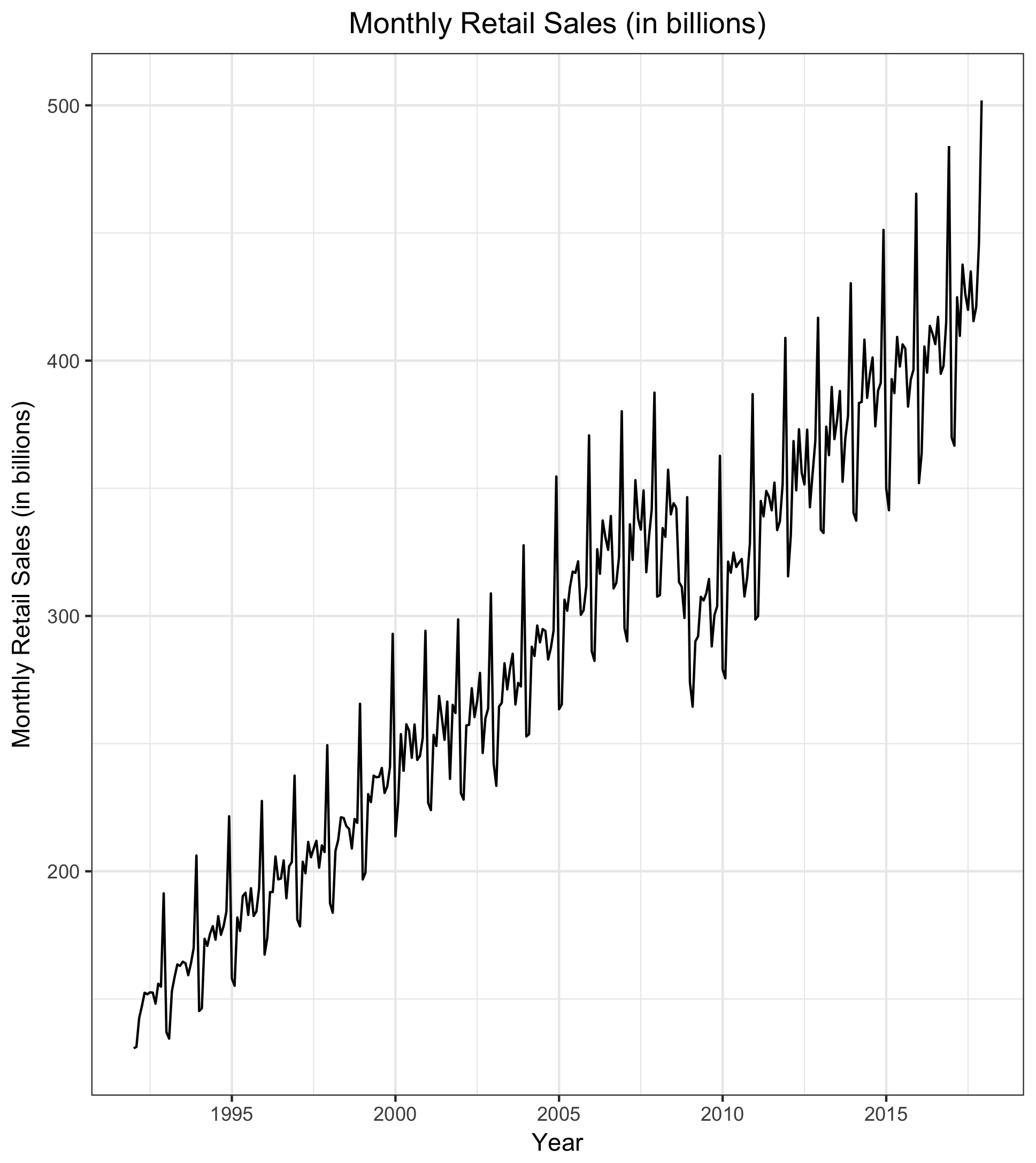
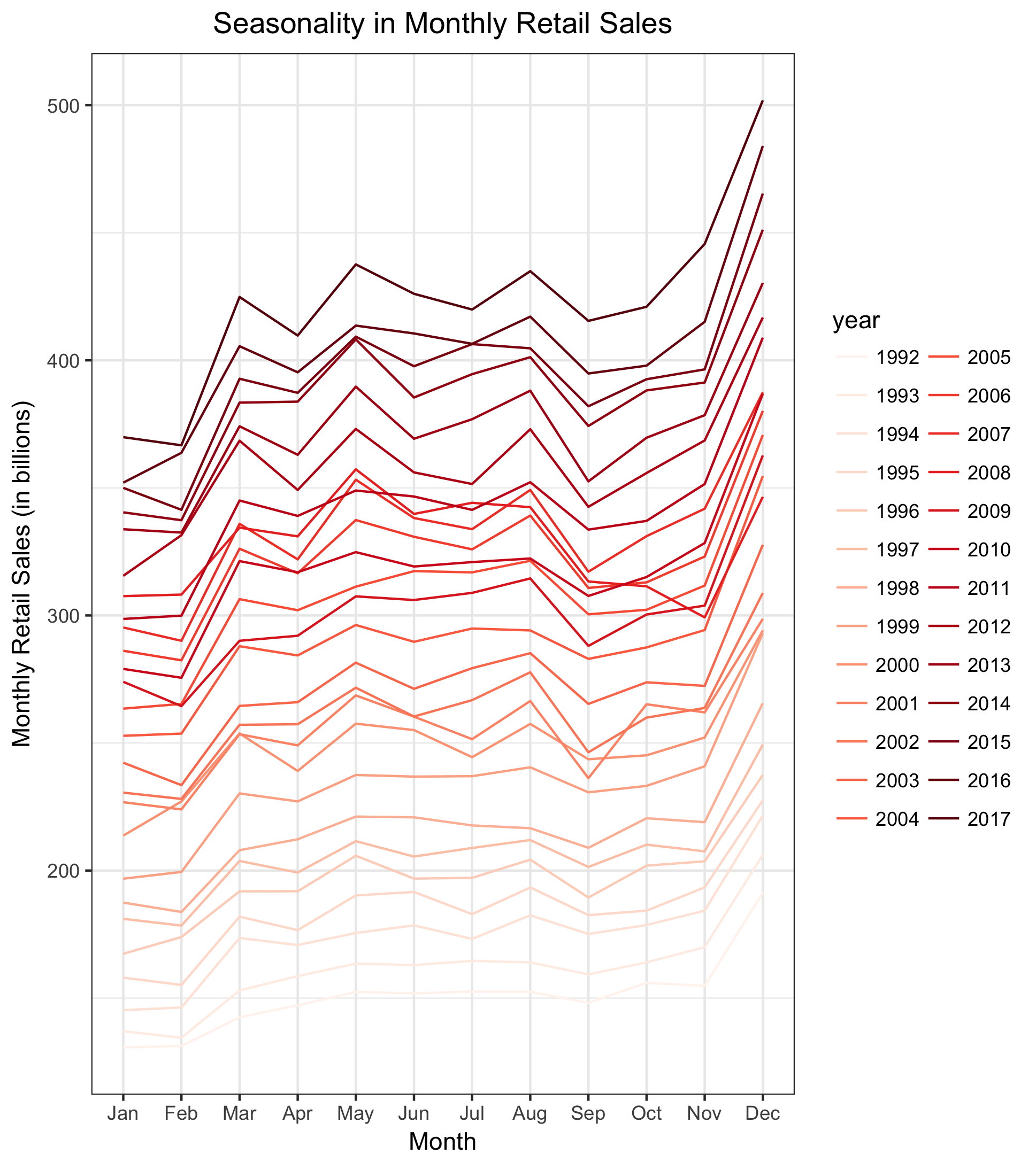
I begin by visually examining characteristics of the monthly retail sales time series. The time series plot indicates a clear upward trend and seasonality in the series. The seasonal plot indicates that retail sales are highest in December and November and lowest in January and February. Forecasting models must account for both the apparent trend and seasonality. In addition, there is a clear dip in sales corresponding with the late-2000s financial crisis, though sales steadily rebound in the 2010s.
### Define universal graphics options used repeatedly throughout analyses
test_xlim <- xlim(2013.000 , 2018.000)
title_center <- theme(plot.title = element_text(hjust = 0.5))

### Plot
plot_sales <- autoplot(ts[,"SALES"], ts.colour = "black") +
  labs(title = "Monthly Retail Sales (in billions)",
       x = "Year",
       y = "Monthly Retail Sales (in billions)") +
  theme_bw() +
  theme(plot.title = element_text(hjust = 0.5))
print(plot_sales)
seasonplot_colors <- brewer.pal(9, "Reds")
seasonplot_colors <- colorRampPalette(seasonplot_colors)(26)
plot_seasonality <- ggseasonplot(ts[,"SALES"], col = seasonplot_colors) +
                    labs(title = "Seasonality in Monthly Retail Sales",
                         x = "Month",
                         y = "Monthly Retail Sales (in billions)") +
                    theme(plot.title = element_text(hjust = 0.5))
print(plot_seasonality)
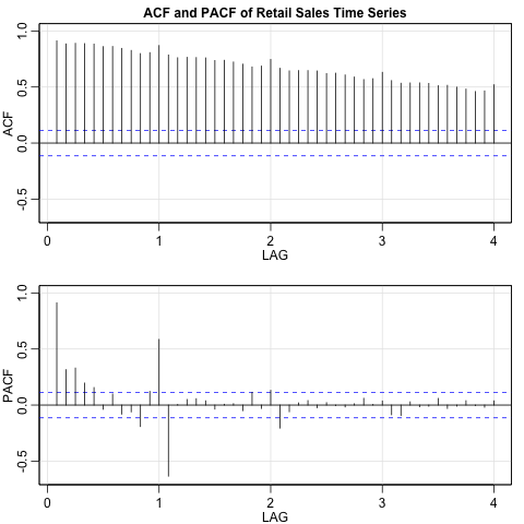
Lastly, the slow decay evident in the ACF indicates the likely presence of a unit root. Augmented Dickey-Fuller and KPSS tests confirm this. Both the ACF and PACF also indicate clear seasonality, in line with prior findings.
Naive Forecast
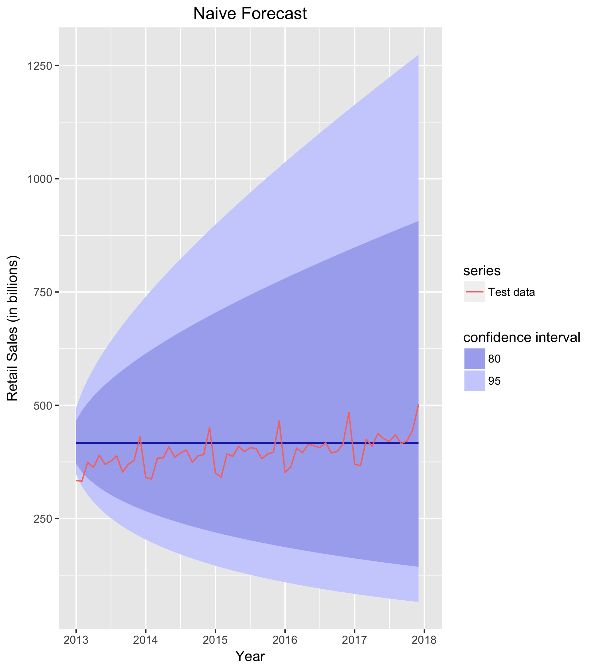
I begin with the most simplistic forecasting method for these data: the naive forecast. Where Yt is the final observation in the training data, the naive method forecasts all future values of the series to be Yt. Because this method simply sets all forecast values to the value of the last observed point in the series, it should miss out on the observed trend and seasonality in the retail sales series.
Before fitting and evaluating the naive forecast, I specify the Box-Cox lambda parameter that will be used in many of the forecasting models. The time series plot clearly shows that the variance increases with the level of the series; in such cases, a transformation is often useful to stabilize the variation in the series. Box-Cox transformations perform this task well. Of course, when forecasting, we must back-transform the data so that the forecasts are on the scale of the original data. Thankfully, the forecast package handles these back-transformations easily. For more detail on Box-Cox transformations, see Hyndman and Athanasopoulos’ exceptional text on time series forecasting.
sales_lambda <- BoxCox.lambda(ts[,"SALES"])
With the transformation specified, I can now implement the naive forecast. I use data from 1992 to 2012 to train all models and reserve observations from 2013 to 2017 for testing the accuracy of each forecasting method. I implement the naive forecast as follows.
naiveSALES <- naive(train[,"SALES"], h = 60, lambda = sales_lambda)
naive_plot <- autoplot(naiveSALES) +
              forecast::autolayer(test[,"SALES"], series = "Test data") +
              labs(title = "Naive Forecast",
                   x = "Year" ,
                   y = "Retail Sales (in billions)",
                   fill = "confidence interval") +
              test_xlim +
              title_center
print(naive_plot)

accuracy(naiveSALES, test[,"SALES"])
As seen in the forecast plot below, the naive forecast expectedly performs poorly, as it misses the seasonal variation and trend in the series (Note: For all forecast plots, the black line is the forecast and the red line is the observed test data). To quantify this inaccuracy, I examine the forecast’s mean absolute error (MAE), which (as the name suggests) takes the mean of the absolute value of the forecast errors. MAE is a common method for evaluating forecast accuracy because of its interpretability, but it should be noted that other valuable metrics also exist (such as RMSE, root mean squared error). The MAE for the naive forecast is 32.29. On average, the forecast errs from the observed test data by $32.29B. This is not ideal; a better forecasting model needs to account for the peculiarities of the time series that the naive method fails to account for.
Lastly, it is important to note that the traditional training/test split is not the only way to evaluate forecasting methods. Time-series cross-validation (TSCV) also provides a robust method for evaluating a foreast. TSCV uses multiple one-observation test sets, where forecast accuracy is computed by averaging over the test sets. For instance, we would use:
- Observation 1 to forecast Observation 2
- Observations 1 and 2 to forecast Observation 3
- Observation 1, 2, and 3 to forecast Observation 4
- And so on…
Of course, we could also examine forecasts that are more than one step ahead. 6-step forecast, for instance, would follow the following pattern:
- Observation 1 to forecast Observation 7
- Observations 1 and 2 to forecast Observation 8
- And so on…
I use training/test sets for these analyses instead of TSCV because TSCV is computationally intensive, especially on long time series. Further, because the retail time series is rather lengthy, training/test sets perform well. Here, I can train the models using 20 years of monthly data and still have 5 years of data to evaluate forecasts. Nonetheless, TSCV could be implemented for the above series. For instance, using the aforementioned RMSE for evaluating forecast accuracy:
ROOTsq <- function(u){sqrt(u^2)}
for (h in 1:12) {
     ts[,"SALES"] %>% tsCV(forecastfunction = naive, h = h) %>%
     ROOTsq() %>% mean(na.rm = TRUE) %>% print()
}
Holt-Winters Forecast
I next implement a Holt-Winters (HW) forecast. The HW method uses exponential smoothing whereby forecasts are a function of past observations, with more recent observations weighted more than observations from the more distant past. Additionally, the HW forecast should improve upon the naive forecast because it appropriately models the observed trend and seasonality in the retail sales series. Importantly, seasonality in a Holt-Winters method can take one of two forms: additive or multiplicative. An additive model is appropriate when the seasonal variability is constant across all levels of the series, whereas a multiplicative model is appropriate when variability changes with the level of the series. As previously discussed, the latter is true of the retail sales series. Thus, I implement a multiplicative model here:
hwSALES <- hw(train[,"SALES"], h = 60, seasonal = "multiplicative")
hw_plot <- autoplot(hwSALES, series = "Forecast") +
           forecast::autolayer(test[,"SALES"], series = "Test data") +
           labs(title = "Holt-Winters Multiplicative Forecasts",
                x = "Year" ,
                y = "Retail Sales (in billions)",
                fill = "confidence interval") +
           test_xlim +
           title_center
print(hw_plot)
accuracy(hwSALES, test[,"SALES"])
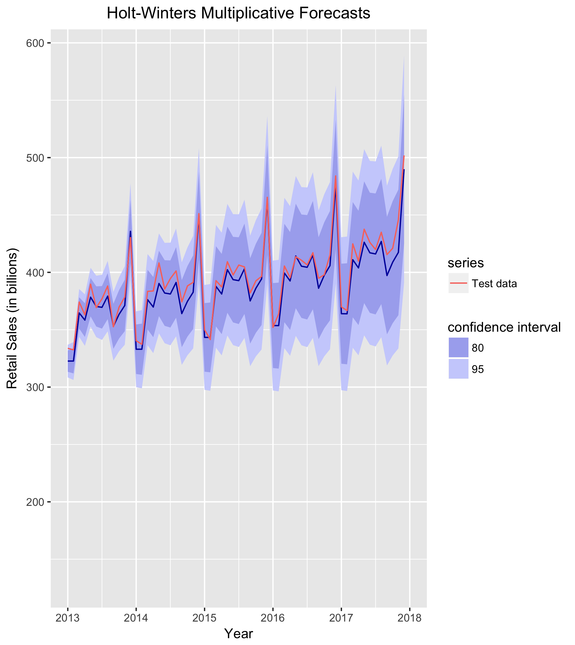
Based solely on the forecast plot, it is immediately apparent that the HW forecast significantly outperforms the naive forecast. It clearly accounts for both the trend, and perhaps more importantly seasonality, in the series. Indeed, the MAE is much better for this forecast as well. Whereas the MAE was $32.29B for the naive forecast, it is only $7.45B for the HW model. On average, the HW forecast errs from the observed test data by just $7.45B. Seeing as the scale of the data is in the $300B-$500B range, a MAE of roughly $7B is pretty good. Still, I will see if I can produce other forecasts that improve upon the HW model.
ARIMA Forecast
I next use an ARIMA (ARIMA) forecast to see if I can improve upon the HW forecast. ARIMA models with seasonality (sometimes referred to as SARIMA) are notated ARIMA(p,d,q)(P,D,Q)m, where:
- (p,d,q) is the non-seasonal part of the model and (P,D,Q)m is the seasonal part of the model
- p and P denote the non-seasonal and seasonal autoregressive parameters of the model, where past values of the series (Yt-h) are used as predictors of the current value of the series (Yt)
- d and D denote the number of non-seasonal and seasonal differences required to make the series stationary
- q and Q denote the moving average components of the model, where past error values are used as predictors of the current values of the series
- m denotes the seasonal period
I implement the ARIMA using the auto.arima function. This function automatically selects the best fitting ARIMA model by selecting the number of differences required using KPSS unit root tests and then minimizing the AICc.
### Fit ARIMA and check diagnostics
arimaSALES <- auto.arima(train[,"SALES"], lambda = sales_lambda)
png("plot-arima_residuals.png")
checkresiduals(arimaSALES)
dev.off()
mean(residuals(arimaSALES))

### Plot forecast
arimaFCAST <- arimaSALES %>% forecast(h = 60)
arima_plot <- arimaFCAST %>% autoplot() +
              autolayer(test[,"SALES"], series = "Test data") +
              labs(title = "ARIMA(2,1,1)(1,1,2)[12] Forecast",
                   x = "Year",
                   y = "Retail Sales (in billions)",
                   fill = "confidence interval") +
              test_xlim +
              title_center
print(arima_plot)
ggsave("plot-arima_forecast.png")

### Forecast accuracy
accuracy(arimaFCAST, test[,"SALES"])
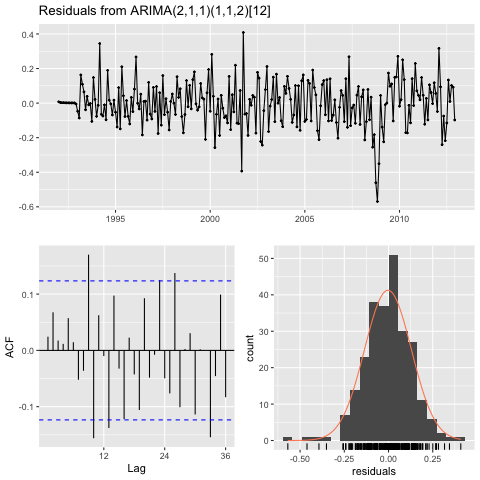
The optimization algorithm selects an ARIMA(2,1,1)(1,1,2)12. Importantly, as seen in the residual diagnostic plots below, the residuals have a mean equal to zero and are at most slightly correlated (except for stronger correlation during the late 2000s recession). Thus, while the residuals are not perfectly white noise, they should suffice for the task at hand here.
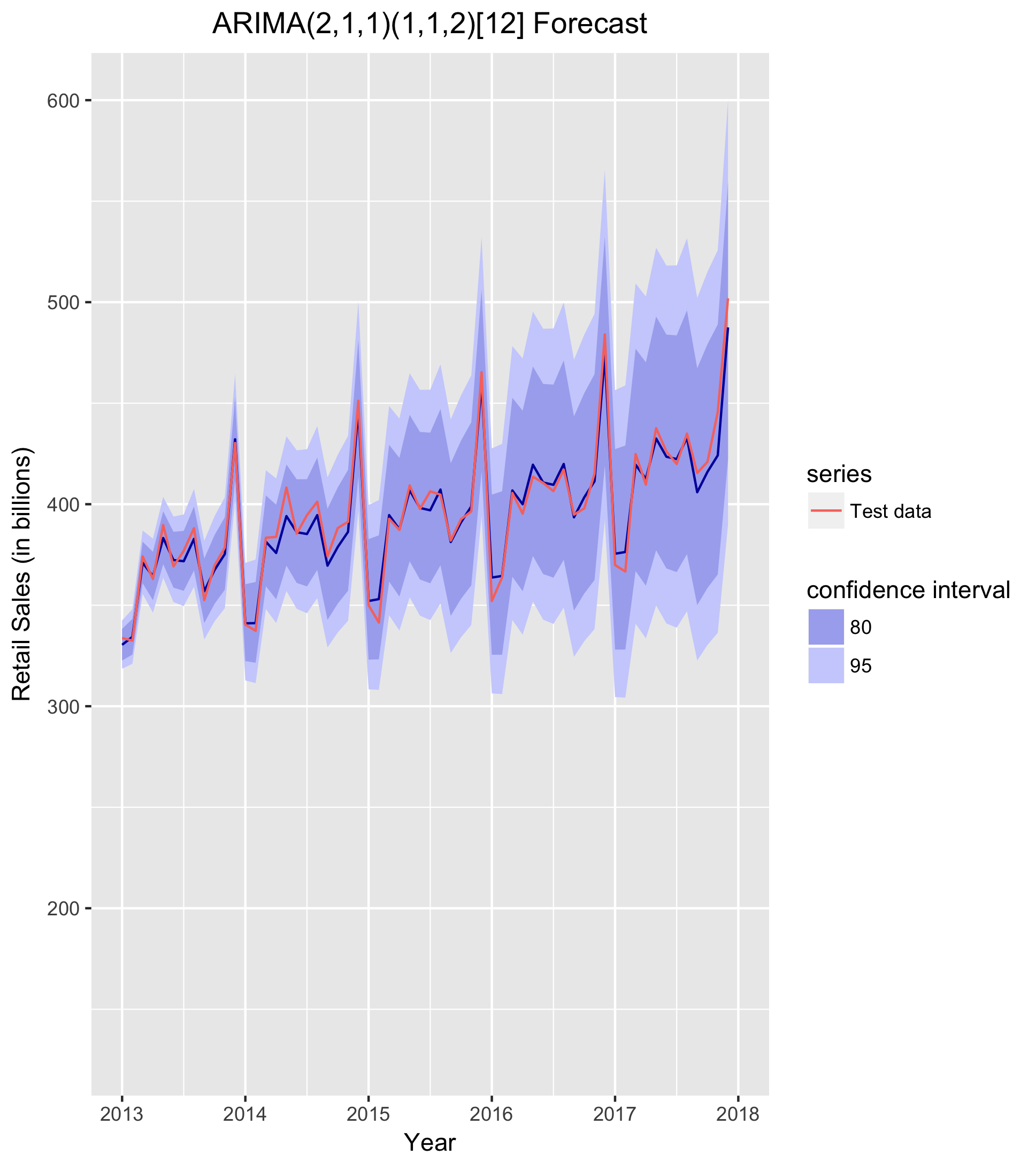
The ARIMA forecast performs spectacularly. While the MAE of $7B was low for the Holt-Winters forecast, it is even lower for the ARIMA forecast: $4.8B. Again, given that monthly retail sales range between $300B-$500B, a mean absolute error of under $5B indicates an incredibly strong forecast. I will attempt to improve upon this as well, but it is a very strong forecasting model as is.
I noted above that the residuals for the ARIMA model are not completely a white noise process. We could, of course, also implement a model that more fully satisfies this essential assumption. In order to do so, we must find a higher order model that more completely picks up the dynamics of the series. I implement a for loop across the non-seasonal and seasonal AR components (p and P) of the model and find the lowest order model that passes the Box-Ljung Q test. The null hypothesis for this test is that the residuals are white noise; thus, we are looking for a p-value above 0.05. The lowest order model that passes formal testing for white noise residuals is an ARIMA(8,1,1,3,1,2)[12].
for (i in 5:10) {
  for (k in 2:4) {
    arimaBL <- forecast::Arima(train[,"SALES"],
                             order = c(i,1,1), seasonal = list(order = c(k,1,2), period = 12))
    checkresiduals(arimaBL)
  }
}

arimaBL <- forecast::Arima(train[,"SALES"],
                         order = c(8,1,1), seasonal = list(order = c(3,1,2), period = 12))

arimaFCASTBL <- arimaBL %>% forecast(h = 60)
arima_plotBL <- arimaFCASTBL %>% autoplot() +
  autolayer(test[,"SALES"], series = "Test data") +
  labs(title = "ARIMA(8,1,1)(3,1,2)[12] Forecast",
       x = "Year",
       y = "Retail Sales (in billions)",
       fill = "confidence interval") +
  test_xlim +
  title_center
print(arima_plotBL)

accuracy(arimaFCASTBL, test[,"SALES"])
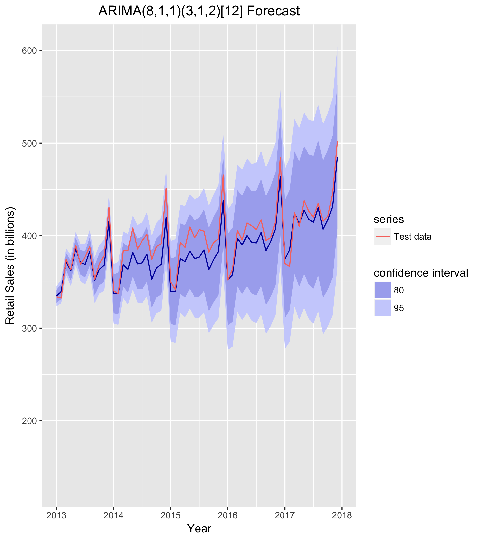
The MAE for the ARIMA(8,1,1)(3,1,2)[12] forecast is $7.6B. Thus, the model is on par with the Holt-Winters forecast, but performs worse than the ARIMA(2,1,1,)(1,1,2)[12] forecast.
Dynamic Regression Forecast
To this point, all for the forecasts have used only the past characteristics of the retail series to predict future values. A dynamic regression model allows external information to be used in calculating forecasts. Here, I use the Consumer Price Index (CPI) as an exogenous regressor predicting retail sales. Thus, I examine whether including changes over time in prices provides valuable forecasting information. Looking at the CPI series, it is clear that it has an upward trend over time.
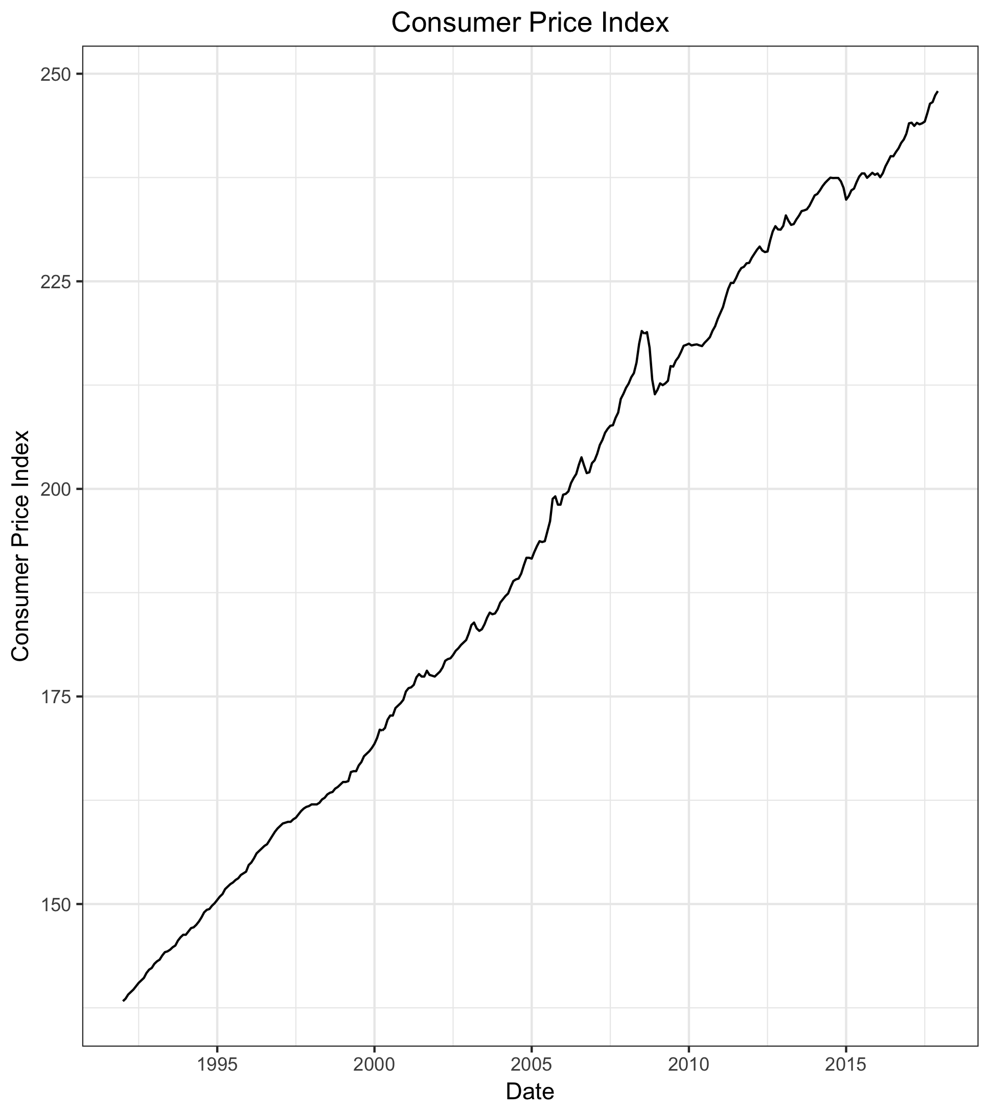
In order to use CPI as an exogenous regressor for the retail sales forecast, I must fit an ARIMA model for CPI using the training data. I must then forecast the CPI series. In doing so, I have forecasted values of CPI that can be used in forecasting retail sales. The best fitting model for the CPI series is an ARIMA(0,1,3)(0,0,1)[12]. I do so as follows:
## Define forecast values for CPI as XREG
cpiFCAST <- auto.arima(train[,"CPI"]) %>% forecast(h = 60)
str(cpiFCAST)

## Fit XREG model
xregSALES <- auto.arima(train[,"SALES"], d = 1, xreg = train[,"CPI"])

## Forecast sales using CPI ARIMA forecast values as XREG
xregFCAST <- xregSALES %>% forecast(h = 60, xreg = cpiFCAST$mean)
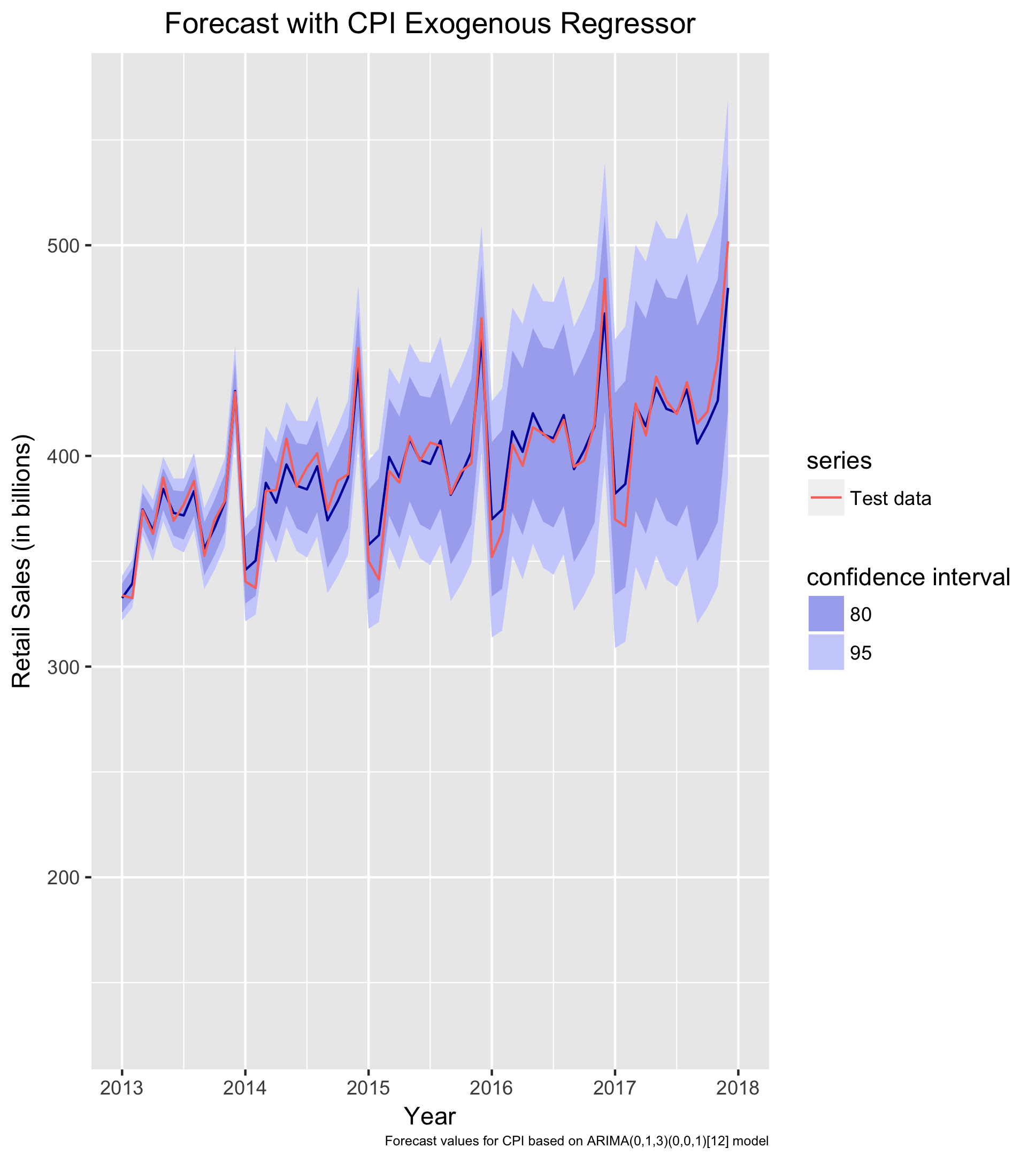
The best fitting model for the retail sales series, including CPI as an exogenous regressor, is an ARIMA(2,1,1)(0,1,2)[12]. Looking at the forecast visualization, the model seems to perform quite well. The forecast performs exceptionally well for 2013 but slowly begins to falter as the forecast range increases. The MAE for this forecast is $6.2B. Thus, while it is not quite as strong as the best performing ARIMA that excludes exogenous regressors, it does outperform the Holt-Winters forecast. All in all, the dynamic regression forecast is quite accurate.
Summary of Findings
I evaluate four forecasting methods for retail sales. Preliminary analyses indicate that the retail sales time series has a clear upward trend and seasonality, both of which must be accounted for in forecasting. The mean absolute errors for the four forecasts are as follows:
| Forecasting Model | Mean Absolute Error (MAE) |
|---|---|
| Naive | $32.29B |
| Holt-Winters | $7.45B |
| ARIMA | $4.80B |
| Dynamic Regression | $6.21B |
The final three forecasts all perform exceptionally well. However, in the end, the ARIMA forecast prevails. A 5-year monthly ARIMA forecast errs, on average, by under $5B. Given that monthly retail sales range from $300-$500B, such a small average error indicates an exceptionally strong forecasting model.
Code for Additional Forecasts
In addition to the forecasts discussed above, I also implemented forecasts using 3 other alternative methods: ETS, dynamic harmonic regression, and TBATS. Each of them performed worse than the ARIMA forecast. To briefly summarize each of these methods:
- ETS is similar to a Holt-Winters model, but uses different optimization methods (see Hyndman)
- Dynamic harmonic regression uses Fourier terms (sines and cosines) to model the periodic seasonality in the series
- TBATS models use trigonometric terms for seasonality, allowing for more complex seasonal modeling
The code to produce these forecasts is below:
# ETS Forecast ------------------------------------------------------------
### Plot
etsSALES <- ets(train[,"SALES"], lambda = sales_lambda)
etsFCAST <- etsSALES %>% forecast(h = 60)
ets_plot <- autoplot(etsFCAST) +
            forecast::autolayer(test[,"SALES"], series = "Test data") +
            labs(title = "ETS(A,Ad,A) Forecast",
                 x = "Year",
                 y = "Retail Sales (in billions)",
                 fill = "confidence interval") +
            test_xlim +
            title_center
ets_plot
ggsave("plot-ets_forecast.png")

### Forecast Accuracy
accuracy(etsFCAST, test[,"SALES"])

# Harmonic Regression Forecast --------------------------------------------
### Find max order of Fourier terms
for (k in 3:6) {
  print(auto.arima(train[,"SALES"], xreg = fourier(train[,"SALES"], K = k),
                   lambda = "auto"))
}

### Plot (using max order = 6 for Fourier terms)
harmonicSALES <- auto.arima(train[,"SALES"], xreg = fourier(train[,"SALES"], K = 6),
                            lambda = sales_lambda)
harmonicFCAST <- harmonicSALES %>% forecast(xreg = fourier(train[,"SALES"], K = 6, h = 60))

harmonic_plot <- harmonicFCAST %>% autoplot() +
                 autolayer(test[,"SALES"], series = "Test data") +
                 labs(title = "Harmonic Forecast with Max Fourier Order = 6",
                      x = "Year" ,
                      y = "Retail Sales (in billions)",
                      fill = "confidence interval") +
                 test_xlim +
                 title_center
harmonic_plot
ggsave("plot-harmonic_forecast.png")

### Forecast Accuracy
accuracy(harmonicFCAST, test[,"SALES"])

# TBATS Forecast ----------------------------------------------------------
### Plot
tbatsSALES <- tbats(train[,"SALES"])
tbatsFCAST <- tbatsSALES %>% forecast(h = 60)
tbats_plot <- tbatsFCAST %>% autoplot() +
              autolayer(test[,"SALES"], series = "Test data") +
              labs(title = "TBATS Forecast",
                   x = "Year" ,
                   y = "Retail Sales (in billions)",
                   fill = "confidence interval") +
              test_xlim +
              title_center
tbats_plot
ggsave("plot-tbats_forecast.png")

### Forecast Accuracy
accuracy(tbatsFCAST, test[,"SALES"])
Updated October 1, 2018
