In this post, I examine and discuss the 4 classifiers I fit to predict customer churn: K Nearest Neighbors, Logistic Regression, Random Forest, and Gradient Boosting. I first outline the data cleaning and preprocessing procedures I implemented to prepare the data for modeling. I then proceed to a discusison of each model in turn, highlighting what the model actually does, how I tuned the model’s hyperparameters, and the results of each model. The best performing model has an out-of-sample test performance of about 80%, and more importantly, an AUC of 0.84. I conclude by comparing the efficacy of the models and discussing avenues by which the models could be improved even further.

NOTE: The following report provides a detailed description of my analyses. To obtain the files used for analysis, see the repository home page.

Contents

Introductory Information
About the Data

Data Cleaning and Analysis
Data Cleaning and Preprocessing
Model 1: K Nearest Neighbors
Model 2: Logistic Regression
Model 3: Random Forest
Model 4: Stochastic Gradient Boosting

Concluding Remarks and Information
Model Comparison and Discussion Areas for Further Improvement

About the Data

Data for these analyses come from IBM. The target feature is customer churn, which is a binary feature “1” if the customer left the company within the last month and “0” if they did not leave in the last month. We have 20 features at the outset that can be used to predict churn, including: whether the customer was a senior citizen, whether they have a partner or dependents, how long they had been customers of the company, monthly charges and other payment information, and whether or not they had several different products through the company (e.g. phone, internet).

Data Cleaning and Preprocessing

I begin by importing all of the packages necessary for data cleaning and analysis and then import the data and store it to the object df.

### Import required packages for preprocessing and analysis
import pandas as pd
import numpy as np
import seaborn as sns
import matplotlib.pyplot as plt
from sklearn.preprocessing import StandardScaler, LabelEncoder
from sklearn.neighbors import KNeighborsClassifier
from sklearn.model_selection import (train_test_split, GridSearchCV, 
                                     RandomizedSearchCV)
from sklearn.metrics import (roc_auc_score, roc_curve, classification_report)
from sklearn.linear_model import LogisticRegression
from sklearn.svm import SVC
from sklearn.ensemble import (GradientBoostingClassifier,
                              RandomForestClassifier)
### Import data                  
df = pd.read_csv('churn.csv')

I then dive into some exploratory data analysis. I start with as broad a scope as possible, looking at generic summary information. The following commands indicate that there are 7043 observations over 21 features, most of which are categorical. The scales of our two continuous features are quite different from each other; customer tenure has a mean of 32 and standard devation of 25, while monthly charges has a mean of 65 and standard deviation of 30 and total charges has a mean of 2283 and standard deviation of 2266. Because some of our classifiers are distance-based (e.g. K Nearest Neighbors), we will need to standardize these features to be on the same scale. I do so later.

### Get preliminary info about dataframe
print(df.info()) # Categorical variables are of type 'object'
print(df.isnull().sum()) # No NaNs

## Set TotalCharges to float 
df['TotalCharges'] = df['TotalCharges'].replace(r'^\s*$', np.nan, regex=True)
df['TotalCharges'] = pd.to_numeric(df['TotalCharges'])

## Set senior citizen to type category
df['SeniorCitizen'] = df['SeniorCitizen'].map({1: 'yes', 0: 'no'}).astype('category')

## Check info of continuous features 
print(df.info()) # Conversion successful
print(df.describe()) # Disparate ranges, should be normalized

I next examine correlations between the continuous features. Because total charges are highly correlated with both tenure and monthly charges, we will remove total charges during feature selection later. In fact, as we see in the correlation between the created variable tenuremonth and TotalCharges, TotalCharges is essentially the multiplication of tenure by MonthlyCharges. Thus, we will retain only tenure and MonthlyCharges as features for modeling.

## Examine correlations
df['tenuremonth'] = (df['tenure'] * df['MonthlyCharges']).astype(float)
df.corr()

## OUTPUT
                  tenure  MonthlyCharges  TotalCharges  tenuremonth
tenure          1.000000        0.247900      0.825880     0.826568
MonthlyCharges  0.247900        1.000000      0.651065     0.651566
TotalCharges    0.825880        0.651065      1.000000     0.999560
tenuremonth     0.826568        0.651566      0.999560     1.000000

I next collapse a handful of the categorical variables related to specific internet services from multiclass to binary. All customers that don’t have a specialized internet service because they don’t have internet service at all are recoded. The same is done for the feature measuring whether the customer has multiple phone lines; if they do not have any phone service at all, their value for multiple phone lines is changed from ‘no phone service’ to ‘no’.

# 6 features, convert 'no internet service' to 'no'
no_int_service_vars = ['OnlineSecurity', 'OnlineBackup', 
                       'DeviceProtection','TechSupport', 
                       'StreamingTV', 'StreamingMovies']
                       
for var in no_int_service_vars:
    df[var] = df[var].map({'No internet service': 'No',
                           'Yes': 'Yes',
                           'No': 'No'}).astype('category')
    
for var in no_int_service_vars:
    print(df[var].value_counts())

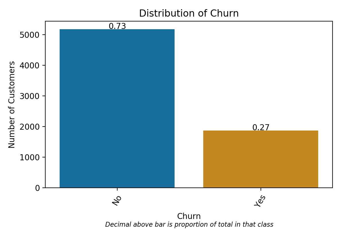
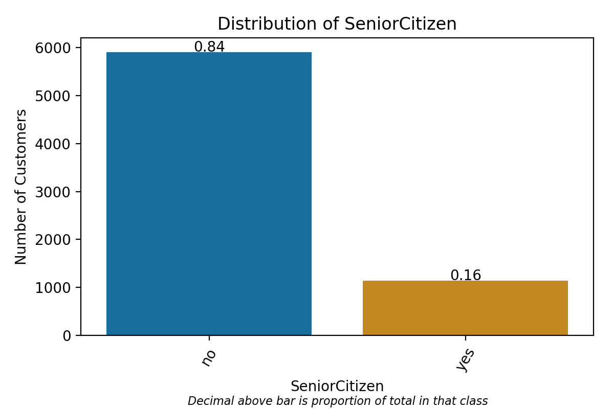
Having done so, I can iterate through all of the categorical variables and plot their distributions. Plots of categorical distributions reveal, for instance, that roughly 27% of customers observed in the dataset churned in the past month and that 16% of customers are senior citizens.

## Define list of categorical variables
cat_vars = ['gender', 'SeniorCitizen', 'Partner', 'Dependents',
            'PhoneService', 'MultipleLines', 'InternetService', 
            'OnlineSecurity', 'OnlineBackup','DeviceProtection', 'TechSupport', 
            'StreamingTV', 'StreamingMovies', 'Contract', 'PaperlessBilling',
            'PaymentMethod', 'Churn']
            
## Plot distributions of categorical variables
for var in cat_vars:
    ax = sns.countplot(x = df[var], data = df, palette = 'colorblind')
    total = float(len(df[var])) 
    for p in ax.patches:
        height = p.get_height()
        ax.text(p.get_x()+p.get_width()/2.,
                height + 10,
                '{:1.2f}'.format(height/total),
                ha="center")
    plt.title('Distribution of ' + str(var))
    plt.ylabel('Number of Customers')
    plt.figtext(0.55, -0.01 , 
                'Decimal above bar is proportion of total in that class',
                horizontalalignment = 'center', fontsize = 8,
                style = 'italic')
    plt.xticks(rotation = 60)
    plt.tight_layout()
    plt.savefig('plot_dist-' + str(var) + '.png', dpi = 200)
    plt.show()

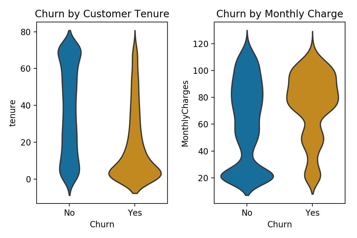
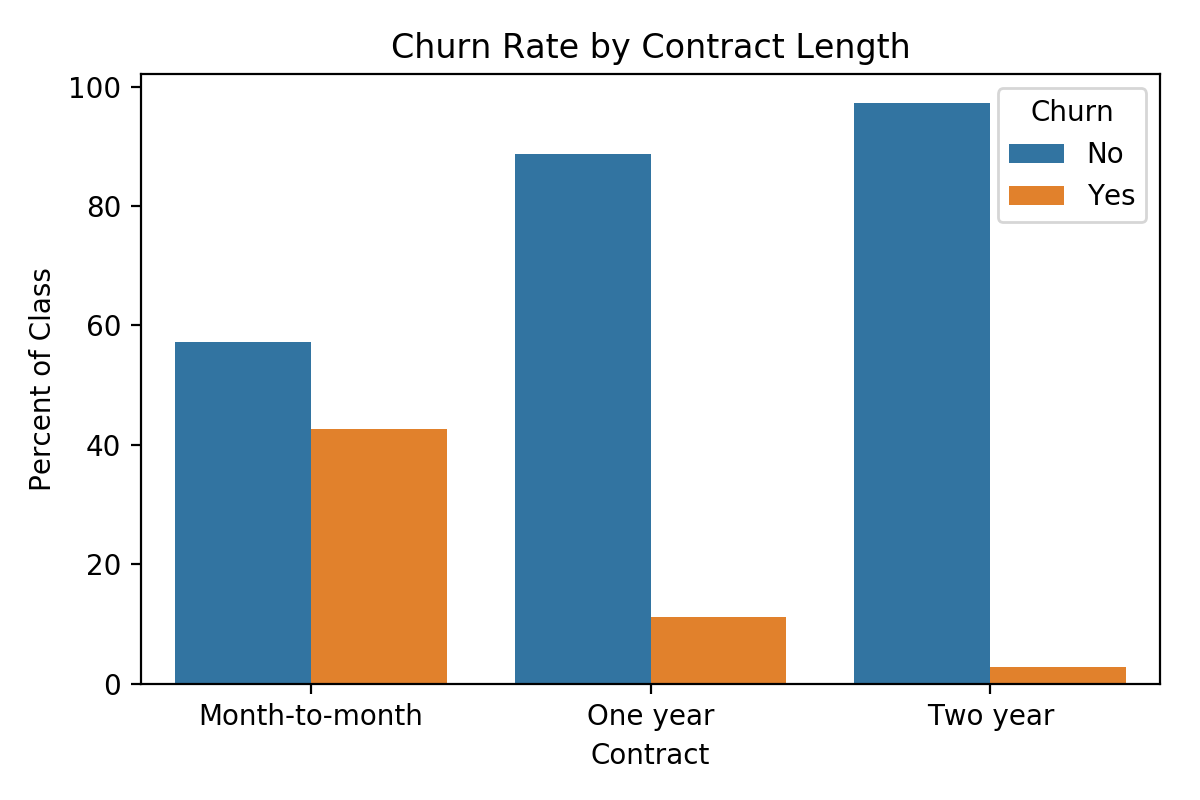
Next, I perform some analyses exploring the distribution of customer churn broken down by features of interest. For instance, violin plots clearly indicate that the bulk of those who churn are relatively new customers and tend to have higher monthly charges. Looking at categorical predictors, we can also see that, for instance, contract length matters quite a bit; about 43% of month-to-month contracts churn, while only 11% of one-year and 3% of two-year contracts do the same. Visualizations of the distributions of all variables (including those not included here), as well as select breakdowns of churn, can be found here.

Now, having explored the data thoroughly, I preprocess the data for analysis. First, as mentioned above, it is necessary to standardize continuous measures so that they are on the same scale. I use StandardScaler from sklearn.preprocessing to do so, transforming each continuous measure to have zero mean and unit standard deviation (sd = 1).

### Standardize continuous variables for distance based models
scale_vars = ['tenure', 'MonthlyCharges']
scaler = StandardScaler() 
df[scale_vars] = scaler.fit_transform(df[scale_vars])
df[scale_vars].describe()

Lastly, I binarize all binary variables using LabelEncoder from sklearn.preprocessing and one-hot encode multi-class categorical variables using get_dummies from pandas. One-hot encoding is one method of preparing categorical variables so that they can be properly utilized by machine learning algorithms. For any categorical variable with some number of levels d, one-hot encoding returns d binary variables, one each for every level of the original multi-class categorical variable. For instance, encoding a categorical measure of political partisanship (Democrat, Republican, Independent, Other) would return 4 binary variables, one each for Democrat, Republican, Independent, and Other.

## Binarize binary variables
df_enc = df.copy()
binary_vars = ['gender', 'SeniorCitizen', 'Partner', 'Dependents',
               'PhoneService', 'MultipleLines', 'OnlineSecurity', 
               'OnlineBackup','DeviceProtection', 'TechSupport', 
               'StreamingTV', 'StreamingMovies', 'PaperlessBilling', 'Churn']
enc = LabelEncoder()
df_enc[binary_vars] = df_enc[binary_vars].apply(enc.fit_transform)

## One-hot encode multi-category cat. variables
multicat_vars = ['InternetService', 'Contract', 'PaymentMethod']
df_enc = pd.get_dummies(df_enc, columns = multicat_vars)
df_enc.iloc[:,16:26] = df_enc.iloc[:,16:26].astype(int)
print(df_enc.info())

Having ensured that the data has been fully pre-processed for analysis, the final step before fitting models is to split the data into training and test sets. I use 70% of the observations for training the models and reserve 30% for testing their out-of-sample performance. Because there is some class imbalance in the target variable – only 1/4 of customers churned – I stratify my train-test split on the target variable. This ensures that roughly 1/4 of the observations in both the training and testing data are customers who have churned.

X = df_enc.drop('Churn', axis = 1)
y= df_enc['Churn']
X_train, X_test, y_train, y_test = train_test_split(X, y, test_size = .3,stratify = y, random_state = 30)

Model 1: K Nearest Neighbors

I begin with one of the simplest, but most interpretable, machine learning models: K Nearest Neighbors (KNN). In short, KNN classifies a given observation O based on the K observations that are most similar to it using a simple majority vote. For instance, in a binary setting where K=9, if 5 of the 9 nearest observations to O are “1” and 4 of the 9 nearest observations to O are “0”, then O is classified as “1”. “Nearest” is determined using one of a several distance metrics; the scikit.learn KNN classifer defaults to Euclidean distance.

I implement KNN using the following code. In addition, I implement grid searching to tune two hyperparameters of the model, K and weights. This allows us to find the most optimal value of for both hyperparameters in order to maximize performance. Grid searching is computationally taxing, so while I use it here for the KNN, computational performance could be sped up using randomized searching (more on that later). Of course, a randomized search is less exhaustive and thus less certain to provide the most optimal hyperparameters, so there is a trade-off here. I also use 5-fold cross-validation to help reduce overfitting the model as much as possible.

knn = KNeighborsClassifier()

## Set up hyperparameter grid for tuning
knn_param_grid = {'n_neighbors' : np.arange(5,26),
                  'weights' : ['uniform', 'distance']}

## Tune hyperparameters
knn_cv = GridSearchCV(knn, param_grid = knn_param_grid, cv = 5)

## Fit knn to training data
knn_cv.fit(X_train, y_train)

## Get info about best hyperparameters
print("Tuned KNN Parameters: {}".format(knn_cv.best_params_))
print("Best KNN Training Score:{}".format(knn_cv.best_score_)) 

## Predict knn on test data
print("KNN Test Performance: {}".format(knn_cv.score(X_test, y_test)))

## Obtain model performance metrics
knn_pred_prob = knn_cv.predict_proba(X_test)[:,1]
knn_auroc = roc_auc_score(y_test, knn_pred_prob)
print("KNN AUROC: {}".format(knn_auroc))
knn_y_pred = knn_cv.predict(X_test)
print(classification_report(y_test, knn_y_pred))

## OUTPUT 
Tuned KNN Parameters: {'n_neighbors': 23, 'weights': 'uniform'}
Best KNN Training Score: 0.7949290060851927
KNN Test Performance: 0.7818267865593942
KNN AUROC: 0.8227581684032563

The grid search selects K = 23 and uniform weights; thus, each observation is classified according to the 23 observations nearest to it, with each of those 23 observations having equal weight in the final classification. Because the best training score during cross-validation (0.795) is close to our out-of-sample test performance (0.782), we can be reasonably confident we did not overfit our model. The area under the receiver operating characteristics curve (AUROC) for the KNN is 0.823. An AUC of 1 indicates a perfect model; an AUC of 0.5 indicates a model that performs no better than a classifier without any information. Thus, we want a model with an AUC as close to 1 as possible. The obtained AUC of 0.823 is a strong start to our classification analyses. To foreshadow, I will discuss AUCs in more detail later when I compare the four classification models.

Model 2: Logistic Regression

I next implement a logistic regression (LR) classifier. We can obtain predicted probabilities from logistic regressions: the probability that any given observation (here: a customer) is “1” (here: churns) given some set of inputs (here: our predictor variables). Stated otherwise, LR gives us P(y=1 | X) for each observation we wish to classify. I reserve a more detailed discussion of decision thresholds until a later discussion of ROC curves. For the purposes of the model accuracy here, if P is greater than 0.5 – that is here, if it is more likely than not the customer churns – the customer is predicted to churn, and vice verse when P is less than 0.5.

I implement the logistic regression as follows. I again use 5-fold cross-validation. Here, I use grid searching to select the optimal value of C, the inverse of regularization strength, where smaller values of C mean more regularization. In short, because coefficients that are large in magnitude can lead to overfitting, regularization penalizes models with large coefficients. This helps combat overfitting the models to our training data and thus helps ensure our models generalize well to unseen data.

## Instantiate classifier
lr = LogisticRegression(random_state = 30)

## Set up hyperparameter grid for tuning
lr_param_grid = {'C' : [0.0001, 0.001, 0.01, 0.05, 0.1] }

## Tune hyperparamters
lr_cv = GridSearchCV(lr, param_grid = lr_param_grid, cv = 5)

## Fit lr to training data
lr_cv.fit(X_train, y_train)

## Get info about best hyperparameters
print("Tuned LR Parameters: {}".format(lr_cv.best_params_))
print("Best LR Training Score:{}".format(lr_cv.best_score_)) 

## Predict lr on test data
print("LR Test Performance: {}".format(lr_cv.score(X_test, y_test)))

## Obtain model performance metrics
lr_pred_prob = lr_cv.predict_proba(X_test)[:,1]
lr_auroc = roc_auc_score(y_test, lr_pred_prob)
print("LR AUROC: {}".format(lr_auroc))
lr_y_pred = lr_cv.predict(X_test)

## OUTPUT
Tuned LR Parameters: {'C': 0.1}
Best LR Training Score:0.8087221095334686
LR Test Performance: 0.7917652626597255
LR AUROC: 0.8340126936435306

Our regularization parameter C is optimal at 0.1. Again, given that the training and test performance are close to each other, there is little concern of overfitting. The area under the receiver operating characteristics curve (AUROC) for the LR classifier is 0.834… an (expected) improvement over the KNN.

Model 3: Random Forest

Random forests are an ensemble method consisting of numerous decision trees. Decision trees start with the target feature of interest and breaks down that feature into subsets by predictors. For instance, in order to break down customer churn, we might draw a tree that splits based on whether the customer is a senior citizen, whether their monthly charge is greater or less than $50, etc. The features used to construct the tree, as well as the cutpoints used to split continuous features, are selected automatically by the learning algorithm. Random forests work because of bagging, wherein subsets of the training data are taken and used to build decision trees. These trees in aggregate create the random forest, which is much more powerful and robust than a single decision tree.

The random forest is implemented as follows. Here, we tune over a large hyperparameter space: n_estimators will find the optimal number of decision trees that should be used to construct the random forest, max_features controls the number of predictor features available to be used when deciding splits for any given decision tree, max_depth controls how deep the tree can grow, min_samples_split controls the minimum number of observations required to produce a split in the tree, and min_samples_leaf finds the minimum number of observations required to be in a leaf node (leaf nodes are the last nodes at the very end of the tree).

 ## Instatiate classifier
rf = RandomForestClassifier(random_state = 30)

## Set up hyperparameter grid for tuning
rf_param_grid = {'n_estimators': [200, 250, 300, 350, 400, 450, 500],
                'max_features': ['sqrt', 'log2'],
                'max_depth': [3, 4, 5, 6, 7],
                'min_samples_split': [2, 5, 10, 20],
                'min_samples_leaf': [1, 2, 4]}

## Tune hyperparameters
rf_cv = RandomizedSearchCV(rf, param_distributions = rf_param_grid, cv = 5, 
                           random_state = 30, n_iter = 20)

## Fit RF to training data
rf_cv.fit(X_train, y_train)

## Get info about best hyperparameters
print("Tuned RF Parameters: {}".format(rf_cv.best_params_))
print("Best RF Training Score:{}".format(rf_cv.best_score_)) 

## Predict RF on test data
print("RF Test Performance: {}".format(rf_cv.score(X_test, y_test)))

## Obtain model performance metrics
rf_pred_prob = rf_cv.predict_proba(X_test)[:,1]
rf_auroc = roc_auc_score(y_test, rf_pred_prob)
print("RF AUROC: {}".format(rf_auroc))
rf_y_pred = rf_cv.predict(X_test)
print(classification_report(y_test, rf_y_pred))

## OUTPUT 
Tuned RF Parameters: {'n_estimators': 400, 'min_samples_split': 20, 'min_samples_leaf': 2, 'max_features': 'log2', 'max_depth': 7}
Best RF Training Score:0.8040567951318458
RF Test Performance: 0.7946048272598202
RF AUROC: 0.8385643502949445

Our hyperparameters are tuned using randomized searching. Here, we randomly search through 20 possible combinations of the hyperparameters and select the best performing combination, which we see in the output. Again, there is little to no concern regarding overfitting here. The AUROC of 0.839 is a slight improvement upon the logistic regression.

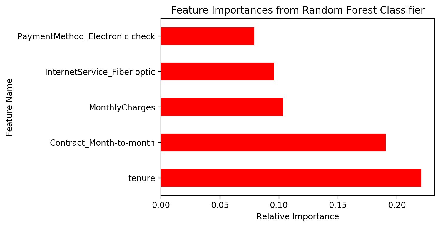
Additionally, one great feature of random forests is that we can extract feature importances. What predictors mattered most in building the forest? The code below produces an easily interpretable chart. We find that, in the random forest model, the length of a customer’s tenure with the company, month-to-month contracts, and monthly charges are the most important features in classifying customer churn.

rf_optimal = rf_cv.best_estimator_
rf_feat_importances = pd.Series(rf_optimal.feature_importances_, index=X_train.columns)
rf_feat_importances.nlargest(5).plot(kind='barh', color = 'r')
plt.title('Feature Importances from Random Forest Classifier')
plt.xlabel('Relative Importance')
plt.ylabel('Feature Name')
plt.savefig('model-rf_feature_importances.png', dpi = 200, bbox_inches = 'tight')
plt.show()

Model 4: Stochastic Gradient Boosting

Gradient boosting is a state-of-the-art ensemble algorithm that often outperforms its competitors. Simply explained, gradient boosting with decision trees is an iterative process, wherein each tree attempts to correct the errors made the preceding tree. Subsequent trees give more weight to observations that are more difficult to predict. On their own, decision trees are not great predictors. But by using all of these “weak learners” (individual decision trees) in tandem, we get a “strong learner”… a strong predictive model.

I tune the gradient boosted tree as follows:

sgb = GradientBoostingClassifier(random_state = 30)

## Set up hyperparameter grid for tuning
sgb_param_grid = {'n_estimators' : [200, 300, 400, 500],
                  'learning_rate' : [0.001, 0.01, 0.05, 0.1, 0.15, 0.2, 0.3, 0.4],
                  'max_depth' : [3, 4, 5, 6, 7],
                  'min_samples_split': [2, 5, 10, 20],
                  'min_weight_fraction_leaf': [0.001, 0.01, 0.05],
                  'subsample' : [0.5, 0.6, 0.7, 0.8, 0.9, 1],
                  'max_features': ['sqrt', 'log2']}

## Tune hyperparamters
sgb_cv = RandomizedSearchCV(sgb, param_distributions = sgb_param_grid, cv = 5, 
                            random_state = 30, n_iter = 20)

## Fit SGB to training data
sgb_cv.fit(X_train, y_train)

## Get info about best hyperparameters
print("Tuned SGB Parameters: {}".format(sgb_cv.best_params_))
print("Best SGB Training Score:{}".format(sgb_cv.best_score_)) 

## Predict SGB on test data
print("SGB Test Performance: {}".format(sgb_cv.score(X_test, y_test)))

## Obtain model performance metrics
sgb_pred_prob = sgb_cv.predict_proba(X_test)[:,1]
sgb_auroc = roc_auc_score(y_test, sgb_pred_prob)
print("SGB AUROC: {}".format(sgb_auroc))
sgb_y_pred = sgb_cv.predict(X_test)
print(classification_report(y_test, sgb_y_pred))

## OUTPUT
Tuned SGB Parameters: {'subsample': 0.8, 'n_estimators': 300, 'min_weight_fraction_leaf': 0.01, 'min_samples_split': 10, 'max_features': 'sqrt', 'max_depth': 6, 'learning_rate': 0.01}
Best SGB Training Score:0.8075050709939148
SGB Test Performance: 0.795551348793185
SGB AUROC: 0.8404496756528291

The optimized model is a stochastic gradient boosted tree model, meaning that a subset of the observations (here, 80% of the training data) are used to fit each tree. Again, there is little concern about overfitting the model here. The AUROC is 0.84, making it the best performing model.

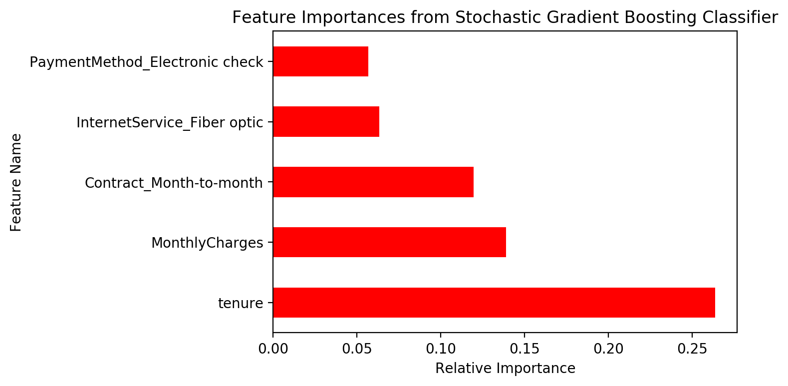
Nicely, we can also examine feature importances from the gradient boosted model. The same 5 features from the Random Forest model are indicated to be the most important features here, albeit in a slightly different rank order.

Model Comparison and Discussion

The four models discussed above are most easily compared examining ROC curves and AUC. ROC curves display the True vs. False Positive Rate of a binary classifier across all decision thresholds (between 0 and 1). In the top right corner is where the decision threshold is 0. In such a case, any observation with a P(y = 1) greater than 0 is classified as a “1”, and the rest are classified as a “0”. Because every observation will satisfy the first condition, every observation is classified as a “1”. Thus, we correctly classify all true “1”s, but incorrectly classify all true “0”s. The converse is true in the bottom left corner, where the threshold is 1. Between these two extremes lie all possible decision thresholds. The area under each ROC curve is known as AUC, which has been referenced many times throughout the post. The ROC curve for the four models discussed here are calculated and plotted as such:

knn_fpr, knn_tpr, knn_thresh = roc_curve(y_test, knn_pred_prob)
plt.plot(knn_fpr,knn_tpr,label="KNN: auc="+str(round(knn_auroc, 3)),
         color = 'blue')

lr_fpr, lr_tpr, lr_thresh = roc_curve(y_test, lr_pred_prob)
plt.plot(lr_fpr,lr_tpr,label="LR: auc="+str(round(lr_auroc, 3)),
         color = 'red')

rf_fpr, rf_tpr, rf_thresh = roc_curve(y_test, rf_pred_prob)
plt.plot(rf_fpr,rf_tpr,label="RF: auc="+str(round(rf_auroc, 3)),
         color = 'green')

sgb_fpr, sgb_tpr, sgb_thresh = roc_curve(y_test, sgb_pred_prob)
plt.plot(sgb_fpr,sgb_tpr,label="SGB: auc="+str(round(sgb_auroc, 3)),
         color = 'yellow')

plt.plot([0, 1], [0, 1], color='gray', lw = 1, linestyle='--', 
         label = 'Random Guess')

plt.legend(loc = 'best', frameon = True, facecolor = 'lightgray')
plt.title('ROC Curve for Classification Models')
plt.xlabel('False Positive Rate (1 - specificity)')
plt.ylabel('True Positive Rate (sensitivity)')
plt.text(0.85,0.75, 'threshold = 0', fontsize = 8)
plt.arrow(0.85,0.8, 0.14,0.18, head_width = 0.01)
plt.text(0.05,0, 'threshold = 1', fontsize = 8)
plt.arrow(0.05,0, -0.03,0, head_width = 0.01)
plt.savefig('plot-ROC_4models.png', dpi = 500)
plt.show()

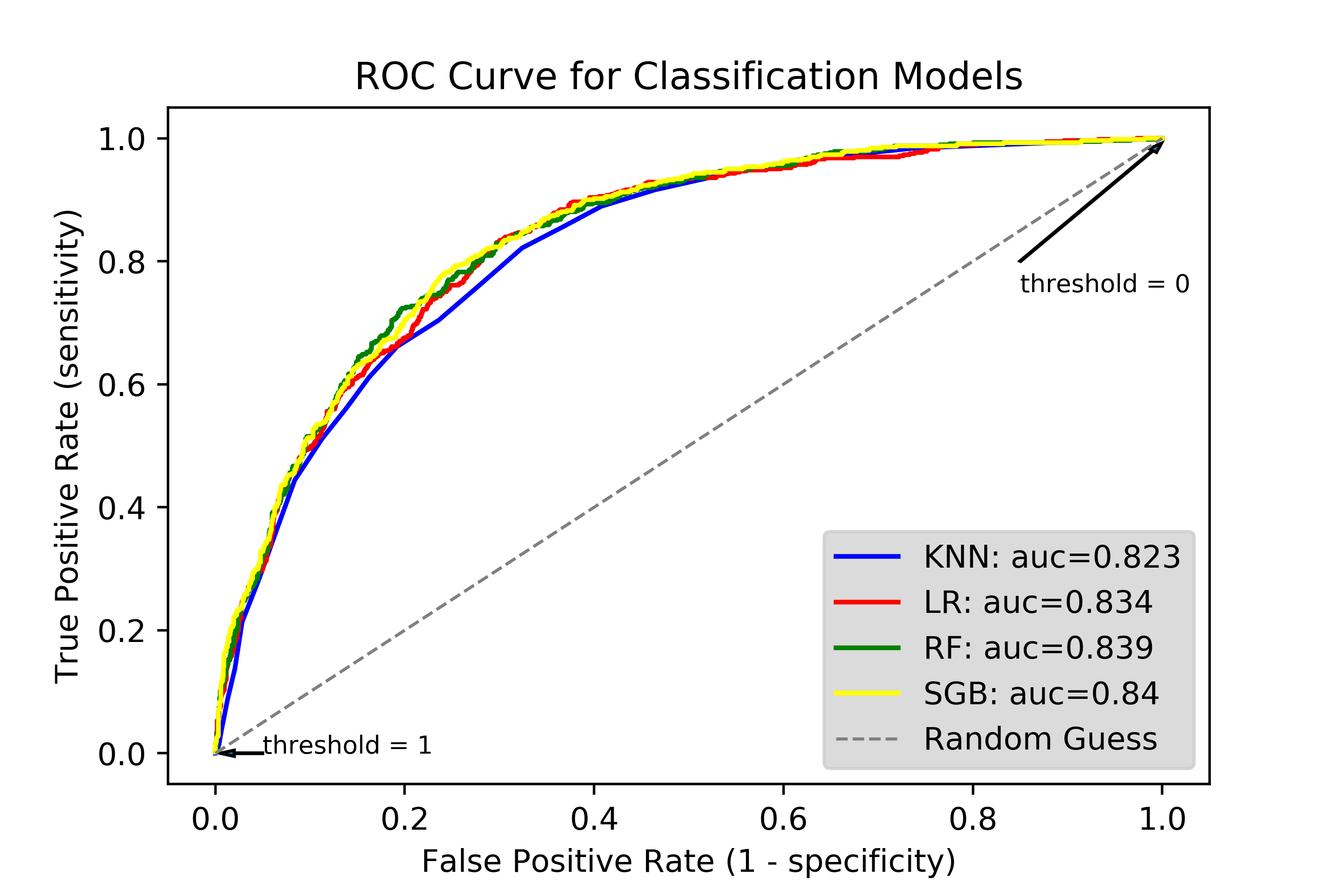
Looking at the areas under the curve, we see that the Stochastic Gradient Boosting (SGB) model performs the best, with an AUC of 0.84; the worst model is the KNN, which has a still-respectable AUC of 0.823. Thus, while there are slight differences in performance across the models, their performance regarding accuracy are generally quite similar.

Of course, we must also consider computational efficiency. For each model, I computed the computation time using the time package. The SGB, though it has the highest AUC, had the longest run time at 111 seconds, whereas the KNN took 98 seconds and the Random Forest took 92. However, the logistic regression was blazingly quick, taking only 1/3 of a second to run. Thus, as a practical matter, the logistic regression model, while slightly worse than the RF and SGB models in terms of AUC, grades out as the best model when taking into account computational efficiency.

Areas for Further Improvement

There are a few avenues that could be investigated further as potential ways of improving model performance. I implemented many data-side preprocessing methods to get the most out of the data at hand, but ideally more refined measures could be collected. For instance, data that measured age as a continuous measure instead of a binary “Senior Citizen” measure would provide the learning algorithms more granular data to work with. Beyond increased data quality, we could of course implement additional preprocessing steps. Though we are working with a relatively limited feature space to begin with, considering dimensionality reduction could prove useful. For instance, given that many features in the data are categorical, the efficacy of correspondence analysis could be evaluated.

Second, more exhaustative hyperparameter tuning could improve model performance to an extent. Of course, expanding the hyperparameter space that we use for GridSearchCV will greatly increase the time required to compute the optimized hyperparameters. Additionally, searching over a larger hyperparameter space does not guarantee that RandomizedSearchCV will settle on the most optimal hyperparameters. If our goal is maximum accuracy regardless of computational intensity, a much more thorough hyperparameter optimization process would likely increase the classification accuracy of the models to some extent. However, the model performances observed using the hyperparameter tuning methods discussed above strike a balance between accuracy and efficiency.

If you’ve made it this far, thank you for reading about my work!

Updated October 4, 2018