Loan Default and Returns on Investment Analyses
In this post, I discuss the logistic regression and random forest classification models I built to predict loan default. I also examine returns on investment as a function of a few key predictors. I find that the logistic regression model slightly outperforms the random forest model with respect to predictive ability. I conclude by discussing the strengths and weaknesses of the discussed models and highlight other pertinent variables that might be used to build a better predictive model.
NOTE: The following report provides an overview of my analyses of loan defaults and ROI. To obtain the files used for analysis, see the GitHub repository home page.
Contents
Introductory Information
Data Source
Data Cleaning and Analysis
Exploratory Analyses
Data Cleaning
Logistic Regression
Random Forest
Return on Investment
Concluding Remarks and Information
Summary of Findings
Limitations and Suggestions for Further Analysis
Data Source
Data for this project is taken from LendingClub’s 2015 publicly available loan statistics. The data contain 127,412 observations on 149 variables, though there are significant patterns of missingness for many of those variables. However, a substantial portion of the missing values are associated with variables that are of little interest for analysis. Importantly, LendingClub’s data includes many variables that are a priori related to loan default. These attributes of the data make it suitable for the analyses I seek to conduct for this project.
Data Cleaning and Analysis
Exploratory Analyses
I begin by examining the distribution of the dependent variable of interest: loan status. For the forthcoming analyses, I treat any loan that’s status is “default”, “charged off”, or “31-120 days” as defaulted (or undesirable) loans and loans that have been fully paid as desirable loans. I thus only examine loans that are, for the most part, “completed”; they have either been closed because of payment (or lack thereof) or are likely to become charged off (loans over 31 days late).
status_keep <- c("Charged Off", "Default","Late (31-120 days)", "Fully Paid")
loan_data_paidORdefault <- loan_data[loan_data$loan_status %in% status_keep,]

loan_data_paidORdefault <- loan_data_paidORdefault %>% mutate(status_bin =
                           factor(ifelse(loan_data_paidORdefault$loan_status == "Charged Off" |
                           loan_data_paidORdefault$loan_status == "Default" |
                           loan_data_paidORdefault$loan_status == "Late (31-120 days)", 1 , 0)))

table(loan_data_paidORdefault$loan_status, loan_data_paidORdefault$status_bin)
                         0     1
                         0     0
  Charged Off            0 17189
  Current                0     0
  Default                0     4
  Fully Paid         47967     0
  In Grace Period        0     0
  Late (16-30 days)      0     0
  Late (31-120 days)     0  1842
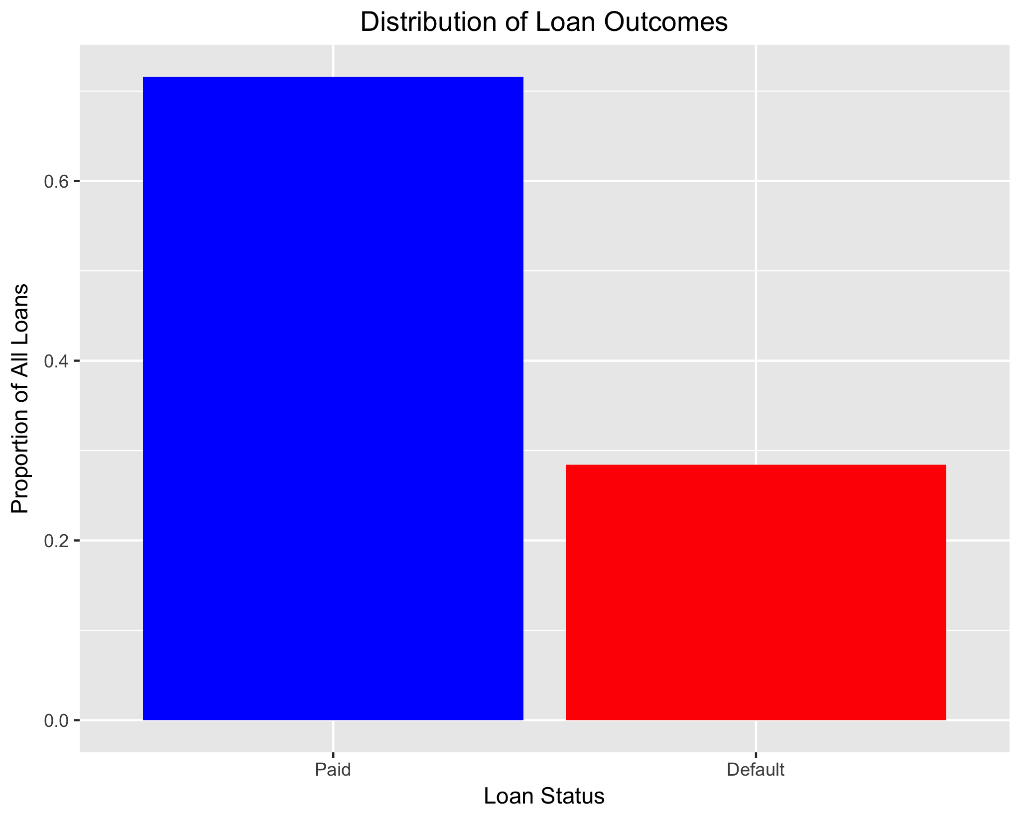
We see that roughly 72 percent of loans in this subset are fully paid and 28 percent have defaulted.
status_dist <- as.data.frame(loan_data_paidORdefault %>%
                               group_by(status_bin) %>%
                               summarise(count = n()))

status_dist$count <- status_dist$count / sum(status_dist$count)

status_dist_graph <- ggplot(status_dist, aes(x = status_bin, y = count)) +
                             geom_bar(stat = "identity", fill = c("blue", "red")) +
                             ggtitle("Distribution of Loan Outcomes") +
                             theme(plot.title = element_text(hjust = 0.5)) +
                             xlab("Loan Status") +
                             ylab("Proportion of All Loans") +
                             scale_x_discrete(labels = c("Paid", "Default")) +
                             scale_fill_discrete(name = "Loan Status", labels = c("Paid", "Default"))
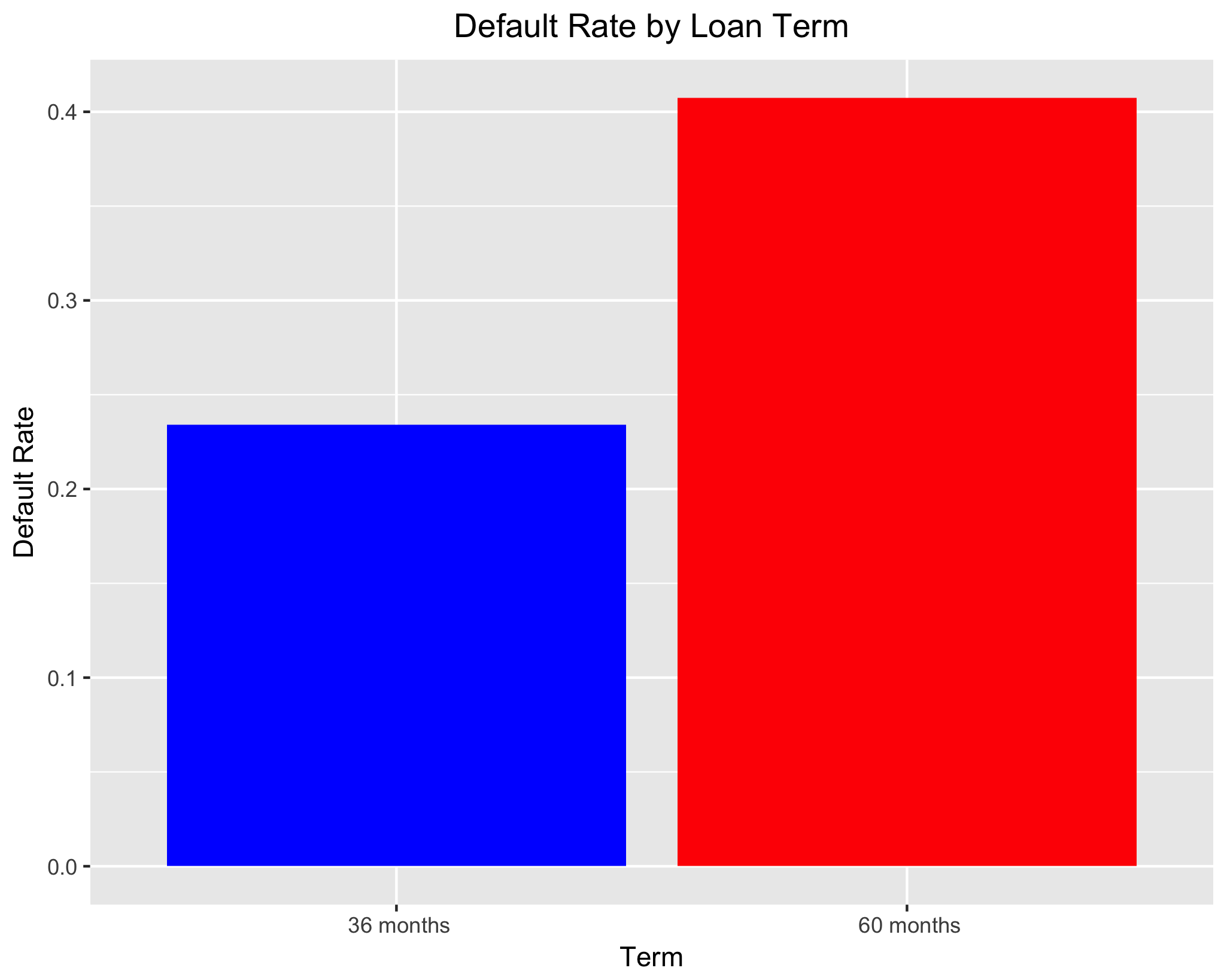
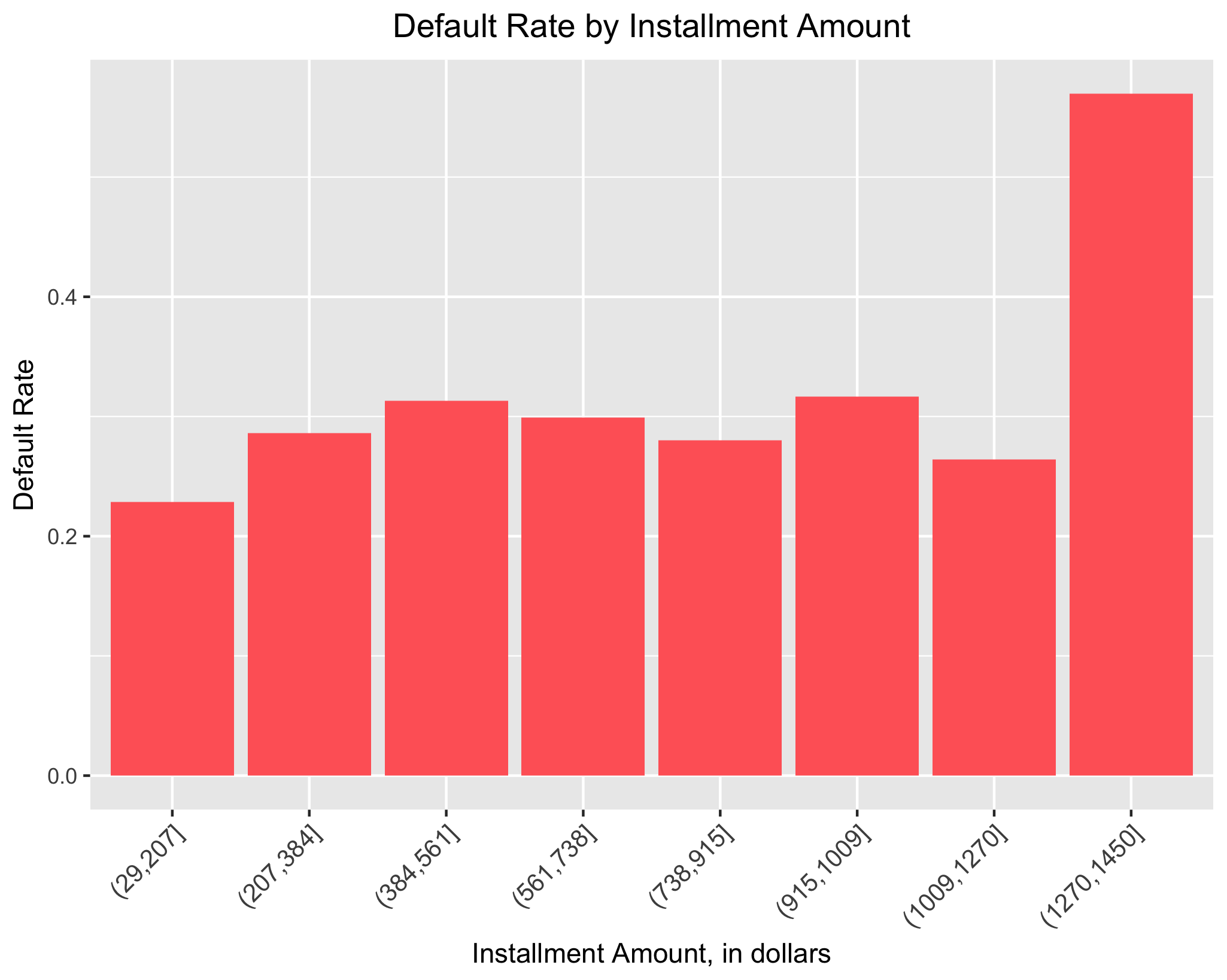
When first examining the data, there are a handful of variables for which a strong theoretical justification for their inclusion in models predicting loan default exists. For instance, one would expect loans with longer terms to be more likely to default because the amount of interest paid – and thus total payments required to pay off the loan –increases as loan terms increase. Similarly, we would expect that as installment amount (the month-to-month payments required for the loan) increases, the likelihood of default would increase as well. Lastly, we would expect a borrower’s grade or subgrade – which are measures of creditworthiness – to be a strong predictor of loan status. Similar to the previous graph, using the group_by and summarise commands from the dplyr package and ggplot2, I examine each of these potential predictors in turn.
As predicted, we see that loan term has a strong impact on the likelihood of default; roughly 41% of 60-month loans default, whereas only about 23% of 36-month loans do. Looking at the graph depicting loan default as a function of installment amount, we some variation. For the lowest 6 installment ranges, default rates range from roughly 23% to 32%. That said, the default rate for the highest installment range is about 57%. It should be noted that alternative specifications for the number of income ranges lead to a similar conclusion.
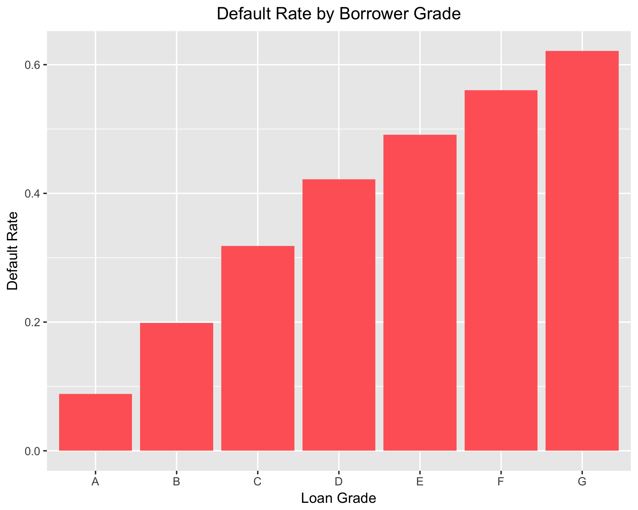
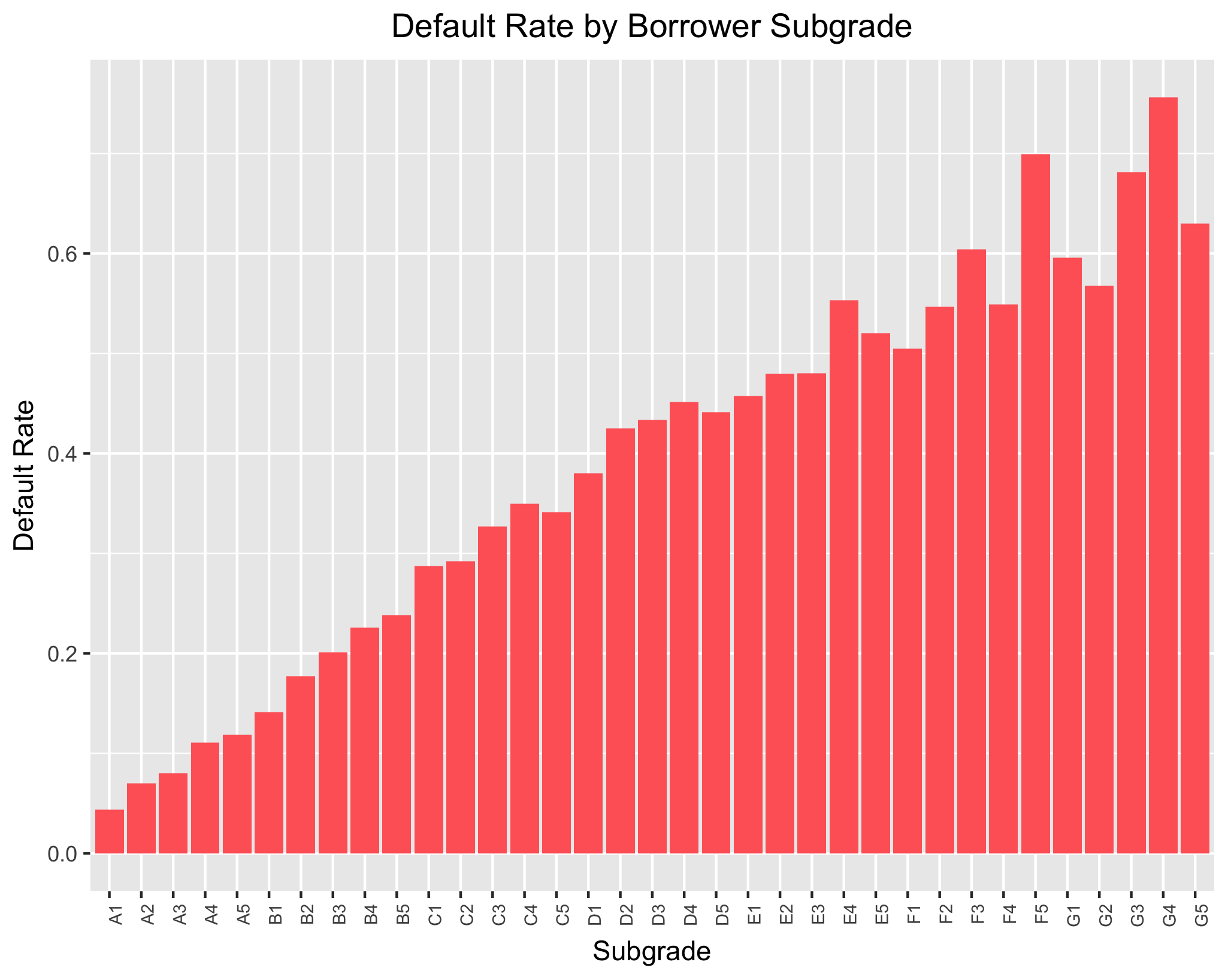
As expected, borrower grade seems to have a large influence on the likelihood of default. Borrower’s graded “A” (those with the most superior creditworthiness) default at the lowest rate and those graded “G” (those with the worst creditworthiness) are the most likely to default. Default rate rises in a roughly linear fashion as you move from “A” to “G”. A similar trend is apparent when looking at borrower sub-grade, which is a more fine-tuned measure of creditworthiness. The least likely sub-grade to default is “A1”, with default rate increasing as borrower creditworthiness gets worse. However, there is a bit of fluctuation evident; for instance, “G4” has a higher default rate than “G5”. That said, both of these exploratory graphs indicate the importance of borrower creditworthiness as a predictor of loan default.
Data Cleaning
Based on these exploratory analyses, I elect to keep these variables, in addition to others that also have strong a priori reasons for being included in my models. Of note, these other variables include debt to income ratio, revolving balance utilization rate, annual income, bankruptcies, and tax liens.
vars_interested <- c("term", "sub_grade", "emp_length", "home_ownership",
                     "addr_state", "application_type", "purpose", "loan_amnt", "installment",
                     "annual_inc", "revol_bal", "revol_util", "total_acc", "dti", "delinq_2yrs",
                     "bankruptcy_bin", "taxliens_bin", "status_bin", "emp_length_num", "sub_grade_num",
                     "total_bc_limit", "total_bal_ex_mort", "num_accts_ever_120_pd",
                     "bc_util", "chargeoff_within_12_mths", "inq_last_12m", "inq_last_6mths","tot_cur_bal",
                     "pub_rec", "ROI", "total_pymnt", "loan_status", "grade")
loan_data_vars_interested <- loan_data_paidORdefault %>% select(one_of(vars_interested))
Logistic Regression Classification Models
I begin by subsetting the data into training and testing sets. I use 75% of the observations for training models and reserve 25% of the observations for testing these same models, setting a seed to ensure reproducibility. In doing so, I can evaluate the “out-of-sample” predictive performance of each model.
loan_clean <- read.csv("loan_data_cleaned.csv")
set.seed(123)
n <- nrow(loan_clean)
train_size <- round(0.75 * n)
train_indices <- sample(1:n, train_size)
train <- loan_clean[train_indices,]
test <- loan_clean[- train_indices,]
I specify Model 1 (M1) using the training data where loan status is a function of the 12 covariates that I initially thought would be the most pertinent. With the exception of the dummy variable indicating whether the loan applicant had a prior bankruptcy, all covariates are statistically significant. However, it should be noted that the magnitude of some of the coefficients is quite small. Additionally, with the exception of “loan amount”, the direction (+/-) of all coefficients is as one would expect. I suspect that the peculiar negative coefficient on loan amount is because of multicollinearity. Checking variance inflation factors (VIF) confirms this; loan amount is understandably highly correlated with installment amount and it appears (to a lesser degree) loan term.
glm(formula = status_bin ~ term + sub_grade_num + emp_length_num +
    loan_amnt + installment + annual_inc + revol_util + total_acc +
    dti + delinq_2yrs + bankruptcy_bin + taxliens_bin, family = "binomial",
    data = train, na.action = na.exclude)

Deviance Residuals:
    Min       1Q   Median       3Q      Max
-3.9024  -0.7940  -0.6049   1.0485   4.5267

Coefficients:
                 Estimate Std. Error z value Pr(>|z|)
(Intercept)    -2.457e+00  5.187e-02 -47.366  < 2e-16 ***
term 60 months  4.735e-01  6.269e-02   7.553 4.26e-14 ***
sub_grade_num   8.030e-02  2.484e-03  32.330  < 2e-16 ***
emp_length_num -1.504e-02  2.935e-03  -5.123 3.01e-07 ***
loan_amnt      -3.756e-05  9.312e-06  -4.034 5.49e-05 ***
installment     1.324e-03  2.960e-04   4.473 7.72e-06 ***
annual_inc     -1.916e-06  3.061e-07  -6.260 3.85e-10 ***
revol_util      3.041e-03  4.796e-04   6.342 2.27e-10 ***
total_acc      -3.378e-03  9.985e-04  -3.383 0.000716 ***
dti             2.204e-02  1.396e-03  15.795  < 2e-16 ***
delinq_2yrs     6.557e-02  1.121e-02   5.847 5.01e-09 ***
bankruptcy_bin  2.446e-02  3.222e-02   0.759 0.447747
taxliens_bin    3.860e-01  5.483e-02   7.040 1.92e-12 ***
---
Signif. codes:  0 ‘***’ 0.001 ‘**’ 0.01 ‘*’ 0.05 ‘.’ 0.1 ‘ ’ 1

    Null deviance: 55759  on 47269  degrees of freedom
Residual deviance: 50959  on 47257  degrees of freedom
  (2982 observations deleted due to missingness)
AIC: 50985

vif(model1)
          term  sub_grade_num emp_length_num      loan_amnt    installment     annual_inc     revol_util
      7.663810       2.094198       1.021674      57.058218      48.372028       1.523804       1.120343
     total_acc            dti    delinq_2yrs bankruptcy_bin   taxliens_bin
      1.284792       1.256508       1.030566       1.054142       1.012880
Based on the above, I specify Model 2 (M2) by removing the covariate for loan amount. I remove this covariate instead of installment amount because there is good reason to believe that installment payments would be more relevant for predicting loan default. It is not just the principal loan amount that should matter, but the month-to-month payments on the principal loan plus interest payments. VIFs for M2 are all at an acceptable level.
I next evaluate the performance of M2 by computing its confusion matrix, using 0.5 as the cut-point for predictions. The model performs slightly better than a model with no information. While the model accurately predicts those that repay their loans relatively well, it misclassifies many defaulted loans as loans that are paid off. In general, the model predicts higher loan repayment rates than is actually observed in the data; whereas there were 4,438 observed defaults in the test data, M2 only predicts 1,442 defaults.
model2_test_prob <- predict(model2, test, type = "response")
model2_test_pred <- as.factor(ifelse(model2_test_prob > 0.5 , 1 , 0))
confusionMatrix(data = model2_test_pred, factor(test$status_bin))
          Reference
Prediction     0     1
         0 10633  3628
         1   632   810
               Accuracy : 0.7287
                 95% CI : (0.7217, 0.7357)
    No Information Rate : 0.7174
    P-Value [Acc > NIR] : 0.0007957
I proceed by specifying Model 3 (M3) adding in more covariates that may be relevant, such as home ownership (mortgage, rent, own) and application type (individual or joint). This additional model highlights more important predictors, such as those previously mentioned.
model3 <- glm(status_bin ~ term + sub_grade_num + emp_length_num +
                           installment + annual_inc + revol_util + total_acc + dti +
                           delinq_2yrs + bankruptcy_bin + taxliens_bin + home_ownership +
                           tot_cur_bal + addr_state + num_accts_ever_120_pd +
                           application_type + inq_last_12m,
                           data = train , family = "binomial", na.action = na.exclude)

**MODEL SUMMARY OMITTED DUE TO LENGTH**

Null deviance: 9561.2  on 7955  degrees of freedom
Residual deviance: 8601.6  on 7890  degrees of freedom
(42296 observations deleted due to missingness)
AIC: 8733.6
I note, however, the pervasive pattern of missingness in this model. Further examination, using the below command, indicates that the variable for the number of credit inquires the applicant had in the 12 months preceding the loan application has tons of missing values. Roughly 83% of the values are missing for this variable. Because of how pervasive this missingness is, I am concerned that the data are missing not at random (MNAR). Conventional methods of handling missing data, such multiple imputation or full-information maximum likelihood, are only appropriate where data is either missing completely at random (MCAR) or missing at random (MAR) (see Dong and Peng 2013). Thus, I determine it is safer to proceed by dropping this covariate from analyses.
sapply(loan_data_vars_interested, function(x) sum(is.na(x)))
I specify the final logistic regression model (M4) by removing the variable with significant missingness and other variables that are statistically significant but have tiny coefficient sizes. This allows me to specify the most parsimonious model wherein the model retains accuracy without becoming overly complex.
model4 <- glm(status_bin ~ term + sub_grade_num + emp_length_num +
                           installment + revol_util + dti + delinq_2yrs +
                           taxliens_bin + home_ownership + tot_cur_bal +
                           addr_state + num_accts_ever_120_pd + application_type,
                           data = train , family = "binomial", na.action = na.exclude)

** SOME OUTPUT OMITTED**

Null deviance: 55759  on 47269  degrees of freedom
Residual deviance: 50286  on 47208  degrees of freedom
(2982 observations deleted due to missingness)
AIC: 50410
First, I note that both M4 and M2 have the same sample sizes and that the AIC is significantly lower for M4 than M2. This is strong evidence that M4 is superior. Further, the confusion matrix indicates that M4 performs slightly better than M2.
model4_test_prob <- predict(model4, test, type = "response")
model4_test_pred <- as.factor(ifelse(model4_test_prob > 0.5 , 1 , 0))
confusionMatrix(data = model4_test_pred, factor(test$status_bin))

Confusion Matrix and Statistics
          Reference
Prediction     0     1
         0 10602  3523
         1   663   915
               Accuracy : 0.7334
                 95% CI : (0.7264, 0.7403)
    No Information Rate : 0.7174
    P-Value [Acc > NIR] : 3.691e-06
                  Kappa : 0.1831
 Mcnemar's Test P-Value : < 2.2e-16
            Sensitivity : 0.9411
            Specificity : 0.2062
Examining the ROC curve, it is clear that M4 performs relatively well, but nonetheless misclassifies many loans.
ROC4 <- roc(test$status_bin, model4_test_prob)
png("graph-ROC_model4")
plot(ROC4, col = "red", main = " Model 4 ROC Curve")
dev.off()

auc(ROC4)
Area under the curve: 0.7208
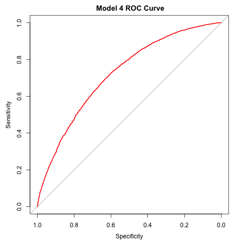
Though M4 is the best performing model considered to this point, it does a poor job of predicting loan default. The model does a great job of accurately predicting loans that are fully paid off; about 94% of loans that are fully paid are predicted to be paid by the model. However, only about 21% of loans that are actually defaulted are predicted to be defaulted by the model. Thus, I also examine the logistic regression classifier using different cut-points for predicting loan default. For instance, classifying all loan applications with a default probability of at least 0.25 as “default” loans leads to a lower overall accuracy rate, but significantly increases the ability of the model to accurately predict loan default. Which cut-point to use should be determined by the lending organization’s goals. If the lender wants to avoid high risk loans as much as possible, a lower threshold for predicting default should be used. While this would decrease the model’s overall accuracy and increase the proportion of desirable loans improperly classified as defaults, it would much better allow the lender to avoid providing loans that would eventually default. For instance, using 0.25 as the threshold, the model accurately predicts 72% of defaulted loans as such – much higher than the 21% predicted using 0.50 as the threshold.
model5_test_prob <- predict(model4, test, type = "response")
model5_test_pred <- as.factor(ifelse(model4_test_prob > 0.25 , 1 , 0))
confusionMatrix(data = model5_test_pred, factor(test$status_bin))

Confusion Matrix and Statistics
          Reference
Prediction    0    1
         0 6839 1258
         1 4426 3180
               Accuracy : 0.638
                 95% CI : (0.6305, 0.6456)
    No Information Rate : 0.7174
    P-Value [Acc > NIR] : 1
                  Kappa : 0.2661
 Mcnemar's Test P-Value : <2e-16
            Sensitivity : 0.6071
            Specificity : 0.7165
Lastly, though the purpose of the logistic regression models is prediction, it is informative to consider the effects of specific covariates in M4. I do so by examining average marginal effects (AMEs). I compute AMEs using the margins package in R. The covariates with the largest influence are application type, home ownership status, tax liens, and loan term. For instance, we see that on average joint applications are approximately 9% less likely to default, individuals who have had a tax lien levied against them are roughly 6.9% more likely to default, and loans with 60 month terms are roughly 5.6% percent more likely to default than loans with 36 month terms.
**AMEs for state of residence omitted for length**

margins4 <-margins(model4, type = "response")
summary(margins4)
                    factor     AME     SE        z      p   lower   upper
 application_typeJoint App -0.0895 0.0273  -3.2781 0.0010 -0.1431 -0.0360
               delinq_2yrs  0.0124 0.0020   6.1021 0.0000  0.0084  0.0163
                       dti  0.0042 0.0002  18.5344 0.0000  0.0038  0.0046
            emp_length_num -0.0016 0.0005  -3.0645 0.0022 -0.0027 -0.0006
         home_ownershipOWN  0.0303 0.0068   4.4429 0.0000  0.0169  0.0437
        home_ownershipRENT  0.0492 0.0051   9.6067 0.0000  0.0392  0.0593
               installment  0.0000 0.0000   4.3632 0.0000  0.0000  0.0001
     num_accts_ever_120_pd  0.0022 0.0014   1.5162 0.1295 -0.0006  0.0050
                revol_util  0.0007 0.0001   8.8611 0.0000  0.0006  0.0009
             sub_grade_num  0.0147 0.0003  43.6586 0.0000  0.0140  0.0153
              taxliens_bin  0.0685 0.0098   6.9817 0.0000  0.0493  0.0877
            term 60 months  0.0555 0.0050  11.1684 0.0000  0.0457  0.0652
               tot_cur_bal -0.0000 0.0000 -12.0445 0.0000 -0.0000 -0.0000
Random Forest Classification Models
I also consider a random forest classifier of loan default. In order to make the best use of the available data, I begin by removing variables that have more than 10% missing values. I also remove any factor variables with more than 32 levels, because R’s random forest classifier cannot handle them. Functionally, this removes the variable for the applicant’s state of residence. I then specify the training and testing sets for analysis.
loan_l10RF <- loan_clean[, ! colMeans(is.na(loan_clean) > 0.10)]
extra_levels <- loan_l10RF %>% lapply(function(x){is.factor(x) == TRUE & nlevels(x) > 32})
loan_dataRF <- loan_l10RF[, extra_levels == FALSE]

nRF <- nrow(loan_dataRF)
train_sizeRF <- round(0.75 * nRF)
train_indicesRF <- sample(1:nRF, train_sizeRF)
trainRF <- loan_dataRF[train_indicesRF,]
testRF <- loan_dataRF[- train_indicesRF,]
I first specify a random forest model using default parameter specifications, which defaults to 4 variables randomly sampled at each split (mtry parameter = 4). The error rate is approximately 27.45%.
set.seed(1)
RFdef <- randomForest(factor(status_bin) ~ . - loan_status - ROI - total_pymnt,
                      data = trainRF,
                      importance = TRUE)

Output:
               Type of random forest: classification
                     Number of trees: 500
No. of variables tried at each split: 4

        OOB estimate of  error rate: 27.45%
Confusion matrix:
      0    1 class.error
0 33381 2607  0.07244081
1 11186 3078  0.78421200
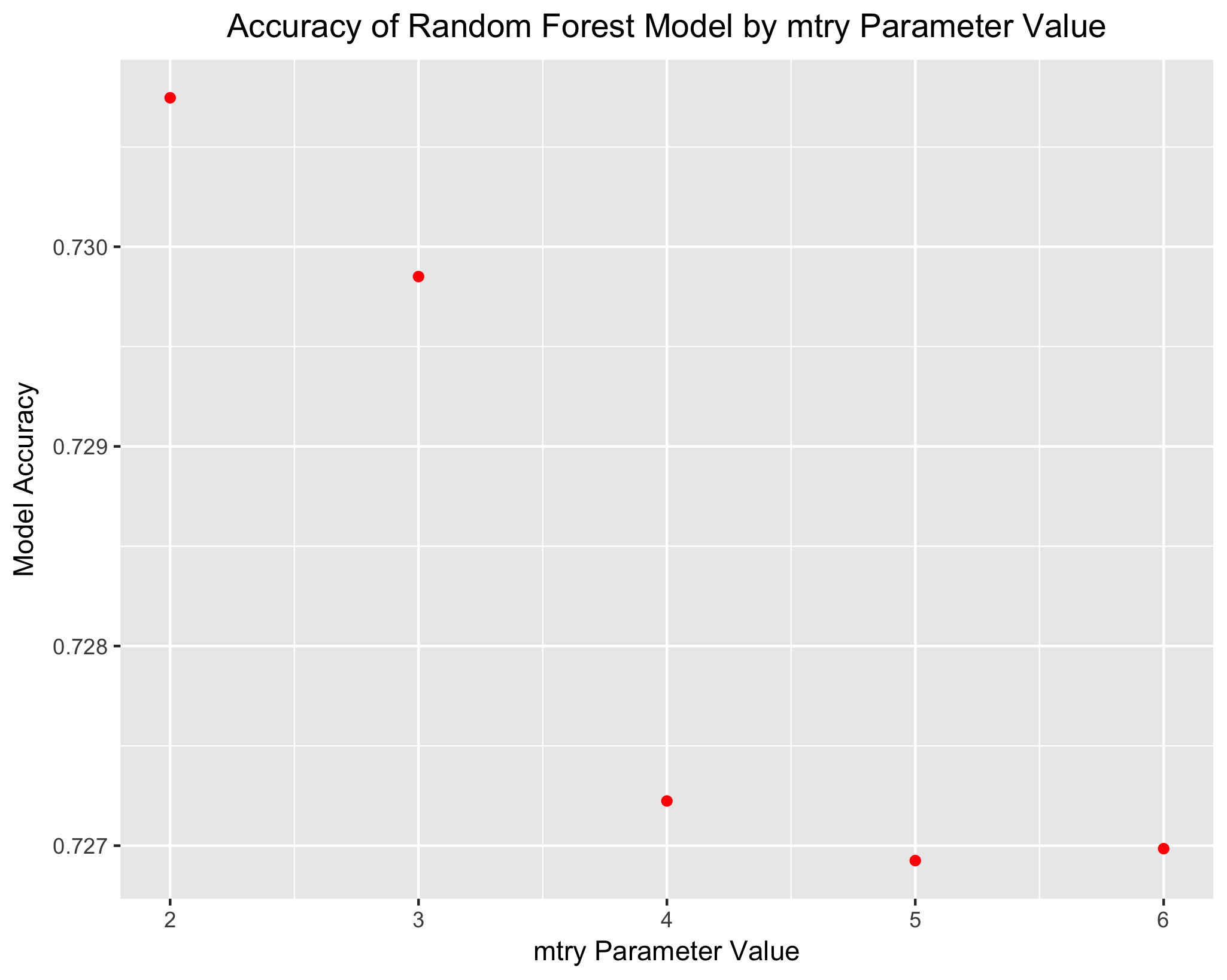
I then implement a for loop to test alternative specifications of the mtry parameter. The most accurate model is that where the mtry parameter is set to 2. The accuracy of this model is 73.07%, which is just barely below the accuracy of the M4 logistic regression model.
set.seed(28)
acc <- c()
for (i in 2:6) {
  RFmtry_i <- randomForest(factor(status_bin) ~ . - loan_status - ROI - total_pymnt,
                           data = trainRF,
                           mtry = i)
  RFmtry_i_pred <- predict(RFmtry_i, testRF, type = "class")
  acc[i-1] = mean(RFmtry_i_pred == testRF$status_bin)
}

acc <- as.data.frame(acc)
print(as.list(acc))
$acc
[1] 0.7307463 0.7298507 0.7272239 0.7269254 0.7269851
Looking at the random forest model with the preferred specification, we can examine the variables with the highest importance. The most important variables include the total current debt balance of the borrower, borrower grade, and revolving credit balance. Interestingly, the random forest model shows that borrower annual income is one of the most important predictor variables; though income was significant in the logistic regression models, the magnitude of the coefficient was quite small.
RF2 <- randomForest(factor(status_bin) ~ . - loan_status - ROI - total_pymnt,
                      data = trainRF,
                      importance = TRUE,
                      mtry = 2)
impRF2 <- as.data.frame(importance(RF2))
impRF2 <- cbind(var = row.names(impRF2), impRF2)
impRF2 <- arrange(impRF2, desc(impRF2$MeanDecreaseAccuracy))
head(impRF2, n = 10)

                 var        0          1 MeanDecreaseAccuracy MeanDecreaseGini
1        tot_cur_bal 39.50902  -6.732374             43.75773        1227.5412
2              grade 32.80298  10.431093             43.19183         794.2698
3          revol_bal 45.39792 -21.321011             39.43266        1166.0611
4      sub_grade_num 28.46259  37.021756             39.29434        1355.1573
5         annual_inc 29.89419   7.879892             37.78732        1116.5008
6          loan_amnt 32.23478 -19.980667             34.12958         936.6649
7        installment 32.31427 -19.333453             34.02163        1117.8835
8     total_bc_limit 32.17642  -1.766777             33.13184        1173.7405
9  total_bal_ex_mort 31.79295 -13.400367             32.59270        1131.3972
10              term 18.89198  10.752782             31.61903         299.8828
Return on Investment
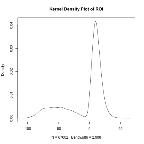
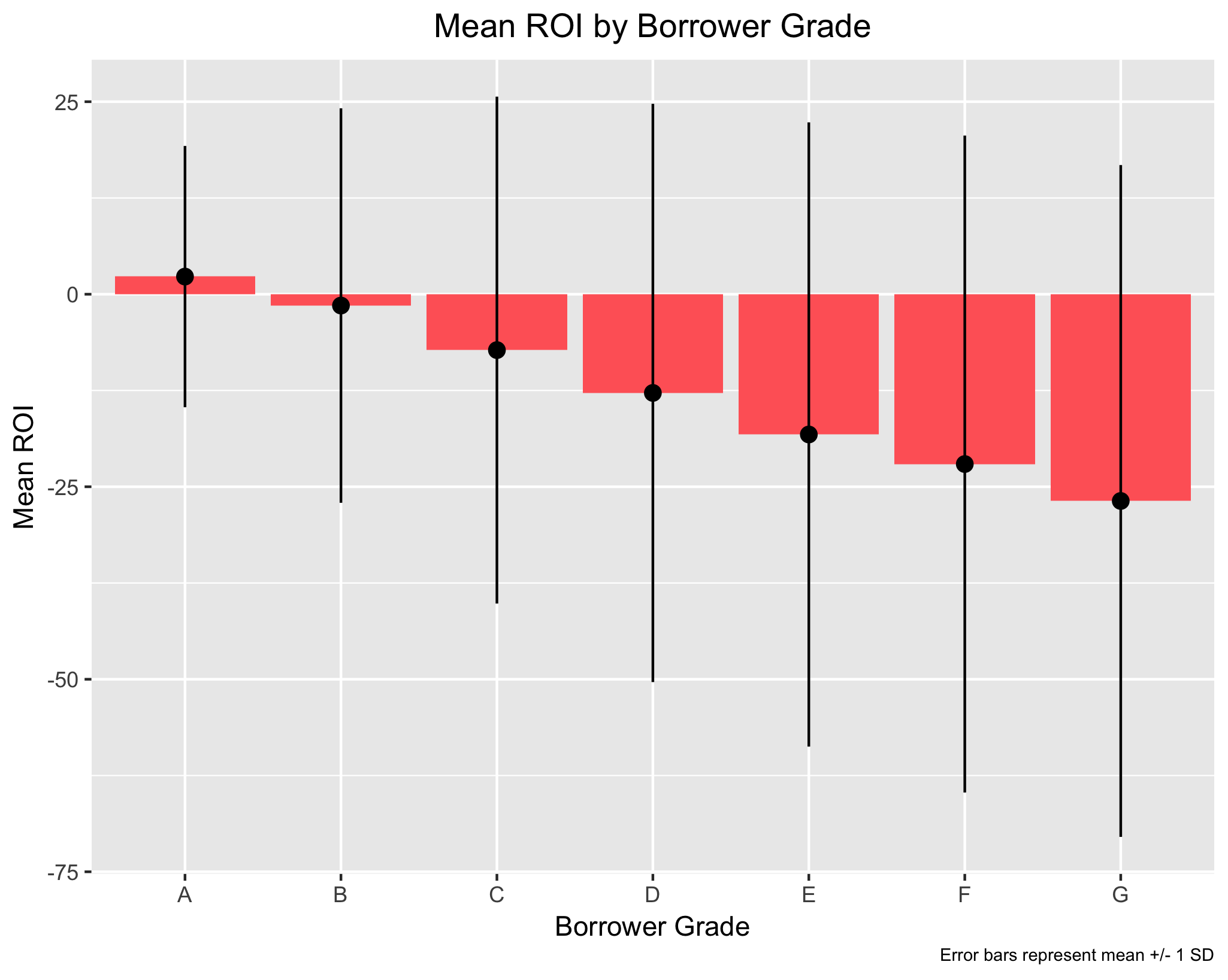
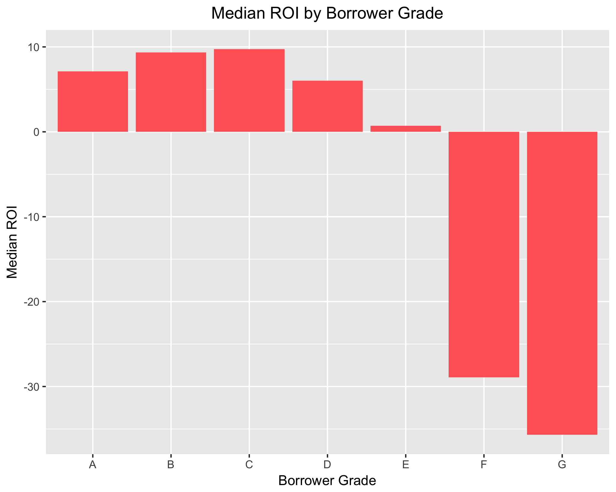
One of the fundamental considerations a bank must consider when deciding whether to approve a loan is whether the loan will provide a solid return on investment (ROI). The last set of analyses I perform for this project considers ROI as a function of a handful of key explanatory variables. First, I consider the distribution of ROI. It exhibits strong negative skew. Because the mean ROI will be heavily influenced by influential low-end outliers (i.e. those with a ROI near -100%), I also examine median ROI.
When looking at ROI by borrower grade, only borrower grade “A” has a mean ROI that is positive. This is unsurprising for two reasons. First, because means are affected significantly by outliers, the numerous low-end values for the lower borrower grades (e.g. “F” and “G”) bring down the mean ROI for those groups significantly. Second, because the data doesn’t look at loans that are “current”, the mean ROI shown here is going to be lower than it perhaps actually is. Many loans that are “current” will eventually become “fully paid”, which would increase mean ROI.
However, median income shows a positive ROI for borrower grades “A” to “E”. When looking at mean and median ROI in tandem, it is clear that a financial institution is most likely to see a positive ROI when the borrower has a higher grade. This is wholly unsurprising.
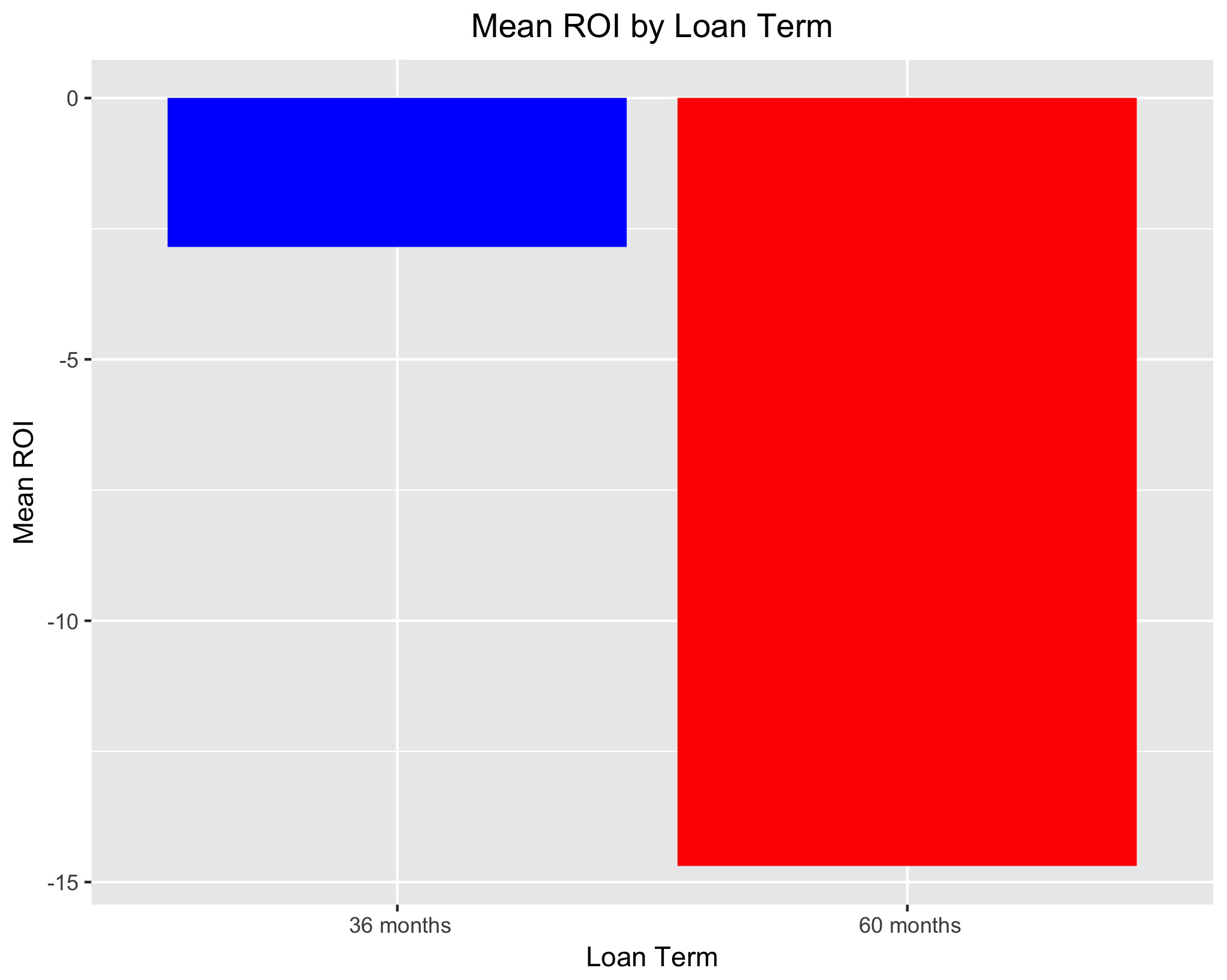
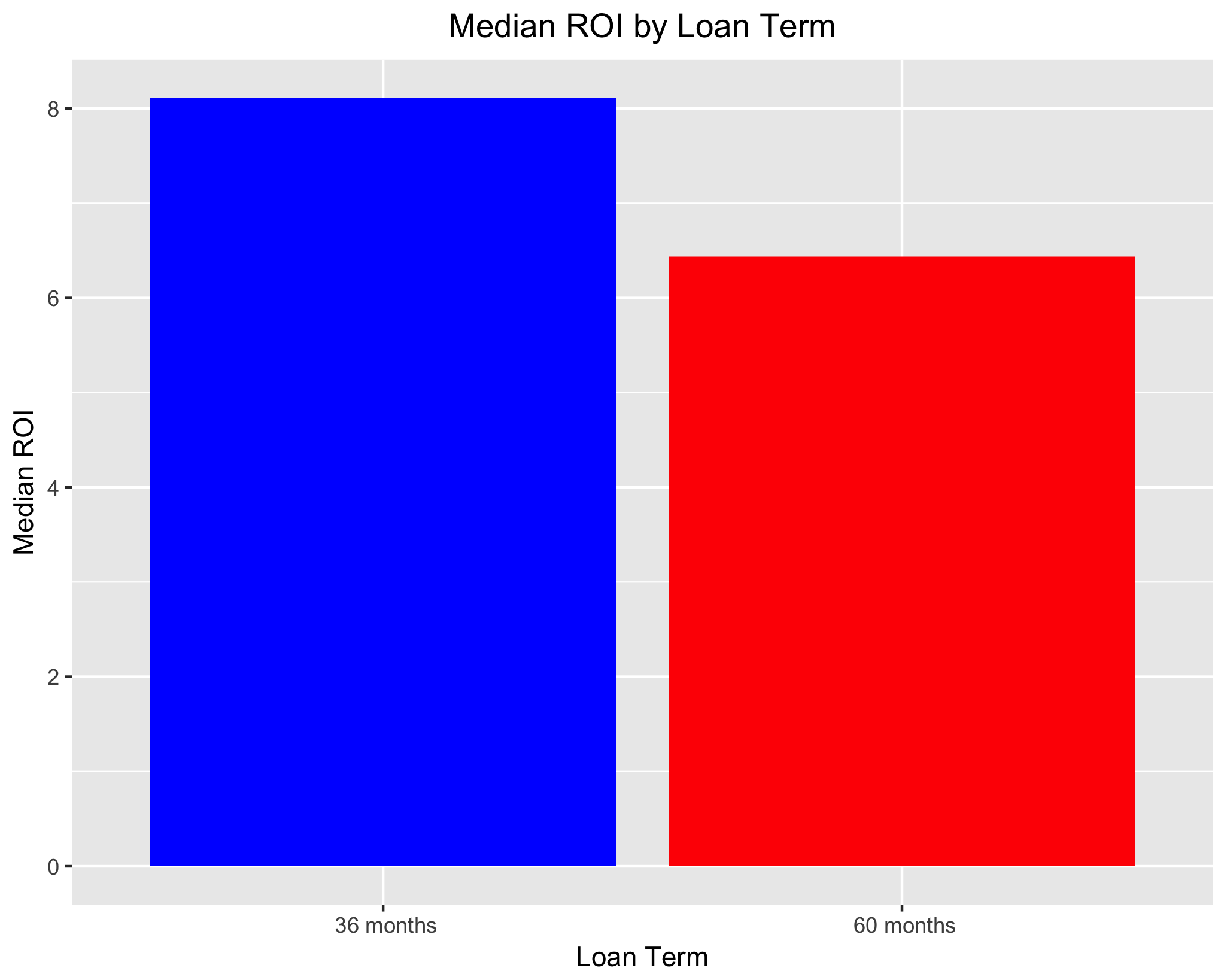
When looking at loan term, we see that mean ROI is negative for both 36 and 60 month loans, whereas median ROI is positive for both loan terms. Perhaps more importantly, both mean and median ROI is higher for 36 month loans. This suggests that, all else equal, a financial institution can be more confident in a strong ROI on shorter-term loans.
Concluding Remarks and Information
Summary of Findings
Exploratory analyses brought to light a handful of covariates that are key predictors of loan default. Relevant predictors of loan default were used to build logistic regression and random forest classification models. Logistic regression performs slightly better than the random forest model, though the difference between the two models in terms of accuracy is marginal. Of note, while the best logistic regression model does exceptionally well with respect to accurately predicting loans that are repaid, it does a poor job of predicting which loans will default. Using a lower threshold for predicting loan default – such as classifying all loans with a 0.25 or greater probability of defaulting as defaults (instead of 0.50) – addresses this shortcoming at the expense of overall model accuracy. The threshold used to classify loans as “paid” or “default” should be decided based on the interests of the lender. If the lender seeks to avoid loan defaults at all costs, a lower threshold will be used. In doing so, the total number of loans approved would be lower because loans would be given only to those indiviudals who the lender is most certain will repay their debt.
Limitations and Further Analysis
Both the logistic regression and random forest classification models perform better than would a model with no information. That said, the covariates in the models presented above only contain characteristics about the loan applicant. Thus, it is important to consider what other information might improve upon these models further. There are two categories of information that would prove valuable here. First, macroeconomic conditions are likely a significant driver of loan default. Default rates, for instance, are certainly higher in times of economic hardship than they are in times of economic prosperity. Thus, analyses that further consider the role of macroeconomic factors beyond the loan applicant’s control are likely to perform better than the one presented here. For instance, an ARIMA model of loan default rates with measures of real or perceived national economic health as exogenous predictors (e.g. unemployment rate or consumer confidence index) would shed light on the role of external factors’ influence on loan default rates.
Additionally, a better predictive model would consider additional sociodemographic characteristics. Of course, it is unlawful to use certain demographic characteristics (e.g. age, race, gender) as the basis for granting a loan or determining interest rates. Nevertheless, other characteristics might be pertinent. For instance, the above models include the applicant’s state of residence. A more refined measure of geographic location, such as zip code, might bring to light other important considerations.
Lastly, I limited the predictor variables in the logistic regression and random forest models to those that I believed had a strong a priori theoretical reason for inclusion in the models. For reasons of computing power, I was intentional in keeping only those variables that I was most confident would be significant in the models. In doing so, it is possible (indeed likely) that I missed important covariates. A more robust predictive algorithm would certainly contain some variables included in the raw data but not in the analytical models presented in this report.
